It all started with the fact that a friend of my friend's friend took assistance with these fetters. Jedi's rumors reached me before me, I unsubscribed in the comments to the link. It seems to help. Well, I hope.
This story stirred in me the memories of the third, or the course, when I myself surrendered to Tsos, and raped writing an article for all those who are interested, how digital filters work, but who is naturally frightened by the Pointed Formulas and Psychedelic Pictures in (I already I'm not talking about textbooks).
In general, in my experience, the situation with textbooks is described by the well-known phrase about the fact that the trees are not visible to the forest. And then say when you are going to scare z-conversion and formulas with division of polynomials, which are often longer than two boards, and interest in the topic runs out extremely quickly. We will start with a simple, the benefit to understand what is happening is completely optional to paint long complex expressions.
So, for a start, a few simple basic concepts.
1. Pulse characteristic.
We put, we have a box with four conclusions. We are without a concept that there is inside, but we know exactly that two left outputs are the entrance, and the two right is the exit. Let's try to apply a very short impulse of a very big amplitude and see what will be at the exit. Well, why, it's like inside this quadrupolymaker, it is unclear because it is not clear to describe it, and so at least something will see.
It must be said here that the short one (generally speaking is infinitely short) the impulse is large (generally speaking, infinite) amplitude in the theory is called a delta function. By the way, the funny thing is that the integral from this infinite Functions is equal to one. Such is normalization.
So, what we saw at the exit of a quadrupolymaker, submitting a delta function, called pulse characteristic This quadrupole. While, however, it is not clear what she helps us, but let's just remember the result obtained and move on to the next interesting concept.
2. Cut.
If we speak short, then the convolution is a mathematical operation that reduces the integration of the product of functions:
![]()
It is indicated, as can be seen, asterisk. It is also seen that when a convolution, one function is taken in its "direct" order, and we are passing by the "backward". Of course, in a more valuable for humanity, a discrete case of a convolution, like any integral, goes into summation:

It would seem that some sad mathematical abstraction. However, in fact, the convolution is perhaps the most magical phenomenon of this world, is surprisingly inferior to only the emergence of a person for light, with the only difference that children come from most people in the most extreme cases for years to eighteen, while about What is a convolution and what it is useful and amazing, a huge part of the population of the Earth does not recognize all their lives.
So, the power of this operation is that if F is any arbitrary input signal, and G is the pulse characteristic of the quadrupole, the result of the convolution of these two functions will be similar to what we would get, passing the signal F through this four-pole.
That is, the pulse characteristic is a complete cast of all the properties of a quadrupolymaker with respect to the input effect, and the input signal bits with it allows you to restore the output signal that corresponds to it. As for me, it's just awesome!
3. Filters.
With a pulse characteristic and a convolution, you can create a lot of interesting things. For example, if the signal is sound, you can organize reverb, echo, chorus, Flanger and a lot, a lot of each other; You can differentiate and integrate ... In general, you can create anything. For us, now the most important thing is that, of course, filters are also easily obtained by convolution.
Actually a digital filter and there is a drill of an input signal with a pulse characteristic corresponding to the desired filter.
But, of course, the impulse characteristic must be somehow obtained. Of course, we have already figured it out above how to measure it, but in such a task it is a bit a bit - if we have already collected a filter, why still measure something, you can use it as it is. Yes, and, in addition, the most important value of digital filters is that they may have characteristics unattainable (or very difficult to achievable) in reality - for example, a linear phase. So there is no way to wash in any way, you just need to count.
4. Obtaining a pulse characteristic.
In this place in most publications on the topic, the authors begin to pour into the reader of the Mount of Z-transformations and fractions of polynomials, confusing it finally. I will not do that, just briefly explain why all this and why in practice for the progressive public it is not much necessary.
Suppose we decided what we would like from the filter, and made a equation that describes it. Further, in order to find a pulse characteristic, you can substitute a delta function to the derived equation and get the desired. The only problem is how to do it, for Delta-function in time aboutthe region is given by a cunning system, and in general there are all infinity. So at this stage everything turns out to be scary.
Here, it happens, and remember that there is such a thing as the Laplace transformation. In itself, it is not a pound of raisum. The only reason that he suffer in radio engineering is the fact that in the space of the argument, the transition to which is this transformation, some things are really becoming easier. In particular, the same delta function is very easily expressed, which delivered so much trouble in the time domain - there is just a unit!
Z-conversion (AKA Laurent transformation) - Laplace conversion version for discrete systems.
That is, applying the Laplace transformation (or z-conversion, if necessary) to a function describing the desired filter, substituting into the received unit and converting back, we get a pulse characteristic. Sounds easily wishing can try. I will not risk, because, as already mentioned, the transformation of Laplace is a harsh thing, especially the opposite. Let's leave it to the extreme case, and we are looking for any simpler ways to obtain the desired one. There are several of them.
First, you can remember about another amazing fact of nature - the amplitude-frequency and impulse characteristics are interconnected by a good and familiar Fourier transformation. This means that we can draw any response to your taste, take the reverse transformation of Fourier from it (at least continuous, even discrete) and get the impulse characteristics of the system that it implements. It's just amazing!
Here, however, it will not be no problem. First, the impulse characteristic that we get, most likely will be infinite (I will not go into explanation why; the world is so arranged), so we will have to trim it at some point (putting equal to zero further). But it will not pass simply as a result of this, as it should be expected, there will be distortion of achm of the calculated filter - it will become a wavy, and the frequency cut will die.
In order to minimize these effects, various smoothing window functions apply to a shortened pulse characteristic. As a result, the response is usually blurred even more, but disappearing unpleasant (especially in the bandwidth) oscillation. 
Actually, after such treatment, we obtain a working impulse characteristic and can build a digital filter.
The second method of calculation is even easier - the impulse characteristics of the most popular filters have long been expressed in the analytical form for us. It remains only to substitute your values \u200b\u200band apply to the result of the window function to taste. So you can not even consider any transformations.
And, of course, if the goal is to emulate the behavior of some particular scheme, it is possible to obtain its impulse characteristic in the simulator:

Here I went to the input RC-chain pulse with a voltage of 100,500 volts (yes, 100.5 kV) with a duration of 1 μs and received its impulse characteristic. It is clear that this is not done in reality, but in the simulator this method, as you can see, works great.
5. Notes.
The above appeal about the shortening of the impulse characteristic was, of course, to the so-called. Filters with a finite impulse characteristic (FIR / ki filters). They have a bunch of valuable properties, including the linear phase (under certain conditions for constructing a pulse characteristic), which gives the absence of signal distortions when filtering, as well as absolute stability. There are filters with an infinite impulse characteristic (IIR / BIH filters). They are less resource-intensive in the sense of calculations, but no longer have listed advantages.
In the next article, I hope to disassemble a simple example of the practical implementation of the digital filter.
Lecture number 10.
"Digital filters with a finite impulse characteristic"
The transfer function of a physically implemented digital filter with a finite pulse characteristic (kih filter) can be represented as
(10.1).
When replacing in the expression (10.1), we obtain the frequency response of the Qih filter in the form of
![]() (10.2),
(10.2),
where ![]() - amplitude-frequency characteristic (ACH) filter
- amplitude-frequency characteristic (ACH) filter
![]() - phase-frequency characteristic (FCH) filter.
- phase-frequency characteristic (FCH) filter.
Phase delay filter is defined as
![]() (10.3).
(10.3).
Group delay filter is defined as
![]() (10.4).
(10.4).
A distinctive feature of the QC filters is the possibility of implementing the permanent phase and group delays, i.e. Linear FCH
(10.5),
where A. - Constant. If this condition is met, the signal passing through the filter does not distort its form.
To display conditions that provide linear FCH write the frequency response of the QC filter, taking into account (10.5)
![]() (10.6).
(10.6).
Equating valid and imaginary parts of this equality, we get
 (10.7).
Sharing the second equation for the first, we get
 (10.8).
Finally you can write down
 (10.9).
This equation has two solutions. First asa. \u003d 0 corresponds to the equation
 (10.10).
This equation has a single solution corresponding to an arbitraryh (0) (sin (0) \u003d 0), and h (n) \u003d 0 for n \u003e 0. This solution corresponds to the filter, the pulse characteristic of which has a single nonzero counting at the initial moment of time. Such a filter represents practical interest.
Another decision will find for. At the same time, crosswise multiple numerators and denominators in (10.8)
(10.11).
From here you have
![]() (10.12).
(10.12).
Since this equation has a view of a Fourier series, its solution, if it exists, is the only one.
It is easy to see that the solution to this equation must satisfy the conditions
(10.13),
(10.14).
From condition (10.13) it follows that for each order of the filterN. There is only one phase delaya. At which the strict linearity of FFH can be achieved. From condition (10.14) it follows that the pulse characteristic of the filter must be symmetrical relative to the point for oddN. , and relative to the midpoint of the interval (Fig.10.1).
 |
Frequency response of such a filter (for oddN. ) can be written as
(10.15).
Making a replacement in the second summ \u003d n -1- n, get
(10.16).
Since h (n) \u003d h (n -1- n ), then two amounts can be combined
 (10.17).
Substituting, we get
(10.18).
If you designate
 (10.19),
then you can finally record
 (10.20).
Thus, for a filter with linear FCH we have
 (10.21).
For the case of evenN. Similarly, we will have
 (10.22).
Making a replacement in the second sum, we get
 (10.23).
Making a replacement, get
(10.24).
Denoted
![]() (10.25),
(10.25),
we will finally have
 (10.26).
Thus, for a Qih filter with linear FCH and even orderN can be recorded
 (10.27).
In the future, for simplicity, we only consider filters with an odd order.
In the synthesis of the transfer function of the filter, the initial parameters, as a rule, are the requirements for frequency response. There are many techniques for the synthesis of kih filters. Consider some of them.
Since the frequency response of any digital filter is a periodic frequency function, it can be represented as a row of Fourier
![]() (10.28),
(10.28),
where the coefficients of the Fourier series are equal
 (10.29).
It can be seen that the coefficients of the Fourier seriesh (N. ) Coincide with the coefficients of the filter pulse characteristics. Therefore, if an analytical description of the desired frequency response of the filter is known, then it can easily determine the coefficients of the pulse characteristic, and on them - the transfer function of the filter. However, in practice, this is not realized, since the impulse characteristic of such a filter has an infinite length. In addition, such a filter is physically implemented as a pulse characteristic begins in -¥ And no ultimate delay will do this filter physically implemented.
One of the possible methods of obtaining a kih filter, the approximating the specified frequency response consists in the truncation of the infinite row of Fourier and the pulse characteristic of the filter, believing thath (n) \u003d 0 at. Then
 (10.30).
Physical implementability of the transfer functionH (Z. ) can be achieved by multiplyingH (z) on.
 (10.31),
where
(10.32).
With such a modification of the transfer function, the amplitude characteristic of the filter does not change, and the group delay increases for a constant value.
As an example, we calculate the low-frequency ki filter with the frequency response
 (10.33).
In accordance with (10.29), the coefficients of the filter pulse characteristics are described by the expression
 (10.34).
Now from (10.31) you can get an expression for gearing function
 (10.35),
where
(10.36).
The amplitude characteristics of the calculated filter for differentN. Presented in Fig.10.2.

Fig.10.2
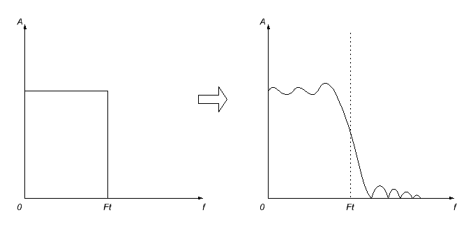
Pulsation in bandwidth and delay bands occur due to the slow convergence of the Fourier series, which, in turn, is due to the presence of a function breaking at the frequency of the bandwidth. These ripples are known as pulsation Gibbs.
Fig.10.2 shows that with increasingN. The pulsation frequency is growing, and the amplitude is reduced both on the lower and at the upper frequencies. However, the amplitude of the last pulsation in the bandwidth and the first ripple in the stroke of the delay remain almost unchanged. In practice, such effects are often undesirable, which requires finding ways to reduce Gibbs ripples.
Truncated pulse characteristich (N. ) can be represented as a product of the required infinite impulse characteristic and some window functions w (n) length n (Fig.10.3).
![]() (10.37).
(10.37).
 |
In the considered case of a simple truncation of the Fourier series used rectangular window
 (10.38).
In this case, the frequency response of the filter can be represented as a complex convolution
 (10.39).
This means that it will be a "blurred" version of the desired characteristic.
The task is reduced to finding the functions of windows to reduce Gibbs pulsations with the same filter selectivity. To do this, it is first necessary to study the properties of the window function on the example of the rectangular window.
Spectrum of the Rectangular Window function can be written as
 (10.40).
The spectrum of the function of the rectangular window is presented in Fig.10.4.

Fig.10.4.
Since, then the width of the main petal spectrum turns out to be equal.
The presence of lateral petals in the spectrum of the window function leads to an increase in Gibbs pulsations in the frequency response. To obtain small pulsations in the bandwidth and large attenuation band in the stroke of the delay, it is necessary that the area limited by side petals makes a small share of the area limited by the main petal.
In turn, the width of the main petal determines the width of the transition zone of the resulting filter. For high selectivity of the filter, the width of the main petal should be as small as possible. As can be seen from the foregoing, the width of the main petal decreases with increasing the order of the filter.
Thus, the properties of suitable windows functions can be formulated as follows:
- the window function must be limited in time;
- the spectrum of the window function should best approximate the function bounded by frequency, i.e. have a minimum of energy outside the main petal;
- the width of the main petal spectrum of the window function should be small.
The most commonly use the following windows features:
1. Rectangular window. Considered above.
2. Hamming window (Hamming).
 (10.41),
where.
With this window is called the Hanna window (hanning).
3. Blackman window (Blackman).
 (10.42).
4. Bartlett window (Bartlett).
 (10.43).
Filter indicators built using the specified window functions are reduced to Table 10.1.
|
Window |
Width of the main petal |
Pulsation coefficient,% |
||
N \u003d 11. |
N \u003d 21. |
N \u003d 31. |
||
|
Rectangular |
22.34 |
21.89 |
21.80 |
|
|
Hanning |
2.62 |
2.67 |
2.67 |
|
|
Hamming |
1.47 |
0.93 |
0.82 |
|
|
Blackman |
0.08 |
0.12 |
0.12 |
|
The pulsation coefficient is defined as the ratio of the maximum amplitude of the side petal to the amplitude of the main petal in the spectrum of the window function.
To select the required order of the filter and the most suitable window function when calculating real filters, you can use the data table 10.2.
|
transient |
Unevenness passing (dB) |
Attenuation B. brokes (dB) |
|
|
Rectangular |
|||
|
Hanning |
|||
|
Hamming |
|||
|
Blackman |
As can be seen from Table 10.1, there is a certain relationship between the ripple coefficient and the width of the main petal in the spectrum of the window function. The smaller the ripple coefficient, the greater the width of the main petal, and therefore the transition zone in the frequency response. To ensure low ripples in the bandwidth, you have to select a window with a suitable ripple coefficient, and to provide the required width of the transition zone to provide an increased order of the filter N.
This problem can be solved using the window offered by Kaiser. The kaiser window feature has a view
 (10.44),
where a is an independent parameter, ![]() , I 0 - Bessel function of the first kind of zero order determined by the expression
, I 0 - Bessel function of the first kind of zero order determined by the expression
 (10.45).
The attractive property of the Kaiser window is the possibility of smooth changes in the ripple coefficient from small values \u200b\u200bto large, when changing only one parameter a. In this case, as for other windows functions, the width of the main petal can be adjusted by the order of the filter N.
The main parameters specified in the development of a real filter are:
Bandwidth - W p;
Broken band - W A;
Maximum allowable pulsation in the bandwidth - a p;
Minimal attenuation in the stroke of the delay - A A;
-sampling frequency -w S.
These parameters are illustrated in Fig.10.5. At the same time, the maximum ripple in the bandwidth is defined as
![]() (10.46),
(10.46),
and minimal attenuation in the stroke of the delay as
A relatively simple procedure for calculating the filter with the Kaizer window includes the following steps:
1. The impulse characteristic of the filter H (n) is determined, provided, the frequency response is ideal
(10.48),
where (10.49).
2. The parameter D is selected as
![]() (10.50),
(10.50),
where  (10.51).
3. The true value A A and A P is currently valid according to formulas (10.46), (10.47).
4. Parameter A as
 (10.52).
5. Parameter D as
 (10.53).
6. The smallest odd value of the order of the filter from the condition
![]() (10.54),
(10.54),
 (10.57)
follows that
Since the filter characteristic samples are coefficients of its transfer function, then condition (10.59) means that the codes of all filter coefficients contain only a fractional part and a sign discharge and do not contain a whole part.
The number of discharges of the fractional part of the filter coefficients is determined from the condition for satisfying the transfer function of the filter with quantized coefficients specified by the requirements for the approximation to the reference gear ratio with the exact values \u200b\u200bof the coefficients.
The absolute values \u200b\u200bof the samples of the filter input signals are usually normalized so that
If the analysis is carried out for a Qih filter with a linear FCH, the algorithm for calculating its output signal may be as follows.
where - rounded to S k coefficients of the filter.
This algorithm corresponds to the block diagram of the filter, shown in Fig.10.5.
 |
There are two ways to implement this algorithm. In the first case, all multiplication operations are performed accurately and the rounding of works is absent. In this case, the size of the works is s in + s k, where S in is the discharge of the input signal, and S k is the discharge of the filter coefficients. In this case, the block diagram of the filter shown in Fig.10.5 exactly corresponds to the real filter.
In the second method of implementing the algorithm (10.61), each result of the multiplication operation is rounded, i.e. Works are calculated with some error. In this case, it is necessary to change the algorithm (10.61) so as to take into account the error made, rounding works
If the countdown values \u200b\u200bof the filter output signal are calculated by the first method (with accurate values \u200b\u200bof works), then the dispersion of the output noise is defined as
![]() (10.66),
(10.66),
those. Depends on the dispersion of the noise of rounding the input signal and the values \u200b\u200bof the filter coefficients. From here you can find the required number of input discharges as
 (10.67).
According to known values \u200b\u200bof S in and S k, you can determine the number of discharges required for the fraction of the output code as
If the values \u200b\u200bof the output signal counts are calculated according to the second method, when each product is rounded to S D discharges, the dispersion of the noise of rounding, created by each of the multipliers can be expressed through the discharge of the work as
DR IN and signal-noise ratio at the output of the SNR OUT filter. The value of the dynamic range of the input signal in the decibels is defined as
![]() (10.74),
(10.74),
where a max and a min is the maximum and minimum amplitudes of the filter input signal.
The signal-to-noise ratio at the outlet of the filter, expressed in decibels, is defined as
![]() (10.75),
(10.75),
determines the mean square value of the output sinusoidal signal filter signal with amplitude A min, and
(10.77)
determines the noise power at the filter output. From (10.75) and (10.76) at a max \u003d 1 We obtain an expression for dispersion of the output noise of the filter
![]() (10.78).
(10.78).
This is the value of the dispersion of the filter output noise can be used to calculate the discharge of the input and output filter output signals.
Consider the simplest of digital filters - filters with constant parameters.
The input signal is fed to the digital filter input as a sequence of numerical values \u200b\u200bfollowing the interval (Fig. 4.1, a). When each next signal value in the digital filter is calculated, the next value of the output signal of the calculation algorithm can be the most diverse; In the calculation process, in addition to the last input signal, the input signal can be used.
previous values \u200b\u200bof the input and output signals: The signal at the output of the digital filter also represents a sequence of numerical values \u200b\u200bfollowing the interval. This interval is one for the entire digital signal processing device.

Fig. 4.1. Input signal and on digital filter output
Therefore, if you submit the simplest signal in the form of a unit pulse to the digital filter input (Fig. 4.2, a)
![]()
then at the output we get a signal in the form of a discrete sequence of numerical values \u200b\u200bfollowing the interval
By analogy with conventional analog circuits, we call this response signal with a pulse filter characteristic (Fig. 4.2, b). In contrast to the impulse characteristics of the analog circuit, the function is dimensionless.

Fig. 4.2. Single impulse and pulse characteristics of the digital filter
Let's give an arbitrary discrete signal to the filter input. 4.1, a), which is a set of discrete values
Under the action of the first element at the output of the filter, a sequence multiplied by a sequence multiplied to and shifted to the right by magnitude, etc. As a result, we obtain a sequence and

Thus, the output signal is defined as a discrete bit of input signal and a pulse characteristic. In this regard, digital filters are similar to conventional circuits, where the output signal is equal to the input signal and the pulse characteristic.
Formula (4.1) is a digital filtering algorithm. If the filter pulse characteristic is described by a sequence with a finite number of members, the filter can be implemented as a scheme shown in Fig. 4.3. Here, the letter indicates the elements of the signal delay at the time (per cell); - elements that multiply the signal to the corresponding ratio.
The diagram shown in fig. 4.3, is not an electrical diagram of a digital filter; This scheme is a graphic image of a digital filtering algorithm and shows a sequence of arithmetic operations performed during signal processing.

Fig. 4.3. Digital Digital Filter Scheme
For digital filters, processing signals in the form of abstract numerical sequences, the concept of "time delay" is not entirely correct. Therefore, elements that delay the signal per cell on digital filter diagrams are usually noted by a symbol indicating the signal delay in the conversion. In the future, we will adhere to this designation.
Let's return to the diagram of the digital filter shown in Fig. 4.3, such filters, where only the input values \u200b\u200bare used to calculate, are called simple or non-neuristic.
The algorithm of the non-ejector filter is easy to record if the pulse filter pulse characteristic is known. For the practical implementation of the algorithm, it is necessary that the pulse characteristic contains a finite number of members. If the pulse characteristic contains an infinite number of members, but they will quickly decrease in magnitude, then it can be limited to a finite number of members, throwing those that are small. If the elements of the pulse characteristic are not declining in magnitude, the non-ejector filter algorithm turns out to be unrealized.

Fig. 4.4. -chain
As an example, consider the simplest digital filter similar to -cepi (Fig. 4.4). Pulse characteristic -cepies
![]()
To record the pulse characteristic of the corresponding digital filter, in the expression should be replaced by however the pulse characteristic of the deck has dimension and the pulse characteristic of the digital filter must be dimensionless. Therefore, we lower the multiplier in the expression (4.2) and write the pulse characteristic of the digital filter in the form of
![]()
Such a pulse characteristic contains infinitely many members, but their value decreases under the exponential law, and can be limited to members, choosing such that
Now you can record the expression for the filter output
This expression is simultaneously the digital filter algorithm. The diagram of this filter is shown in Fig. 4.5.
The second approach to the analysis of processes in digital filters is similar to the operator method of analysis of conventional analog circuits, only instead of the laptose conversion use-conversion.

Fig. 4.5. Scheme of a non-ejective digital filter similar to -cep
Determine the parameter of a digital filter, similar to the transfer function of the electrical circuit. To do this, apply - processing to the pulse characteristic of the digital filter:

The function is called the system function of the filter.
In accordance with the expression (4.1), the signal at the digital filter output is equal to a discrete convolution of the input signal and the filter pulse characteristic. Applying to this expression the theorem about-convert-convection, we obtain that the conversion of the output signal is equal to the conversion of the input signal multiplied by the filter system function:
![]()
Thus, the system function plays the role of the transfer function of the digital filter.
As an example, we find the system function of a first-order digital filter, similar to -cepi:

The third method of analyzing the passage of signals through digital filters is similar to the classical method of differential equations. Consider this method on the example of circuit of order.
The simplest analogue chain of the 1st order is a - with (see Fig. 4.4), the passage of signals through which is described by the differential equation
![]()
For a discrete chain, instead of a differential equation (4.8), a difference equation should be recorded, where the input and output signals are set for discrete moments of time and instead of the derivative, the difference of neighboring signal values \u200b\u200bshould appear. For the discrete chain of the 1st order, the difference equation can be recorded in a rather general form.
Apply to the conversion equation
where you find the system function of the filter
![]()
Formula (4.10) is a fairly common expression for the system function of a digital filter of the 1st order. When it coincides with the previously obtained expression (4.7) for the system function of a digital filter, equivalent to -cepi.
We will find the digital filtering algorithm corresponding to the system function (4.10). To this end, equation (4.9) relative to
The equivalent scheme of this algorithm is shown in Fig. 4.6. Compared to a non-neuristic filter (see Fig. 4.5), a peculiar "feedback chain" was added here, which means that the output values \u200b\u200bare used in the following

Fig. 4.6. Scheme of a recursive digital filter similar to -cepi
calculations. This type of filters are called recursive.
The algorithm (4.11) corresponds to the filter that is completely equivalent to the previously considered non-e-filter. But to determine one value of the output signal using the non-ejective filter (4.4) algorithm (4.4), operations are required, and when using the recursive filter algorithm (4.11), only two operations. This is the main advantage of recursive filters. In addition, recursive filters make it possible to process a signal with higher accuracy, as they allow you to more correctly implement a pulse characteristic without discing its "tail". Recursive filters make it possible to implement algorithms, generally unrealized using non-systemized filters. For example, with a filter that works according to the fig. 4.6, is essentially an ideal drive-integrator and has a pulse characteristic of a form of a filter with such a characteristic on a non-systemic scheme cannot be implemented.
The considered examples show that it makes no sense to apply non-ejective algorithms for creating digital filters with a pulsed characteristic of a large length. In these cases, it is more expedient to use recursive filters.
The scope of non-systemic algorithms is the implementation of digital filters with a pulsed characteristic containing a small number of members. An example is the simplest differentiation, the signal at the output of which is equal to the increment of the input signal:
The diagram of such a digital filter is shown in Fig. 4.7.

Fig. 4.7. Scheme of the simplest digital differential
Consider now a digital filter of a common form, which is described by the equation
This equation can be considered as a difference equation of order and as a digital filtering algorithm if it is otherwise rewritten, namely, namely

Fig. 4.8. Scheme of the recursive digital form filter
The algorithm (4.13) corresponds to the diagram shown in Fig. 4.8. Find the system function of such a filter. To do this, apply to the conversion equation:
Expression (4.14) allows you to establish a link between the chains of the filter circuit elements and the system function. The coefficients in the system function numerator determine the values \u200b\u200bof the coefficients at
(In the non-cross-piece part of the filter), and the coefficients in the denominator determine the recursive part of the filter.
48 Digital filters with a finite impulse characteristic. Calculation of kih filters.
Filter with a finite impulse characteristic (Non-neurous filter, Kih filter) or FIR filter (FIR Socre. from Finite Impulse Response - a finite impulse characteristic) - one of the types of linear digital filters, a characteristic feature of which is the limited time of its pulse characteristic (from some time it becomes exactly equal to zero). Such a filter is also called non-neuristic due to the lack of feedback. An denominator of the transfer function of such a filter is a certain constant.
The difference equation describing the relationship between the input and output signals of the filter: where P.- the order of the filter, x.(n.) - input, y.(n.) - output signal, and b. i. - Filter coefficients. In other words, the value of any reference of the output signal is determined by the sum of scaled values. P.previous samples. You can say otherwise: the filter output value at any time is the value of the response to the instantaneous value of the input and the sum of all gradually dropping responses P.previous signal samples that still affect the output (after P.- flows The pulse transitional function becomes equal to zero, as already mentioned, so all the members after P.-Ho will also become equal to zero). We write the previous equation in a more tank:

In order to find the core of the filter to put
x.(n.) = δ( n.)
where δ ( n.) - Delta function. Then the pulse characteristic of the kih filter can be recorded as:

Z-transformation of the pulse characteristic gives us the transfer function of the Qih filter:

] Properties
The kih filter has a number of useful properties, due to which it is sometimes more preferable to use than a BIA filter. Here is some of them:
Kih filters are stable.
Kih filters during implementation do not require feedback.
Phase kih filters can be made linear
Direct Filter Form
Filters can be implemented using three elements: multiplier, adder and delay unit. The variant shown in the figure is the direct implementation of type 1 kih filters.

Implementation of the direct form of the Filter
Example program
Below is an example of a Kih filter program written in C:
/ * Filter for 128 taps * /
float Fir_FILTER (Float Input)
static Float Sample;
aCC \u003d 0.0F; /* Battery */
/ * Multiplication with accumulation * /
for (i \u003d 0; i< 128; i++) {
aCC + \u003d (H [i] * sample [i]);
/* Output */
/ * Shift the delay signal * /
for (i \u003d 127; i\u003e 0; i--)
sample [i] \u003d sample;
49 Smoothing data. Sliding averaging.
50 data smoothing. Smoothing by parabolami.
51 data smoothing. Spencer smoothing.
52 Smoothing Data. Median filtering.
Sliding averaging, smoothing with trips, smoothing Spencer, median filtering
When developing ways to determine the parameters of physical processes, slowly changing in time, an important task is to eliminate the effect of noise effects or random interference, which are superimposed on the processable signal obtained at the output of the primary converter.
To eliminate such an effect, you can apply data smoothing. One of the most simple ways to such smoothing is arithmetic averaging. When applied, each value of the discrete function (data processable) is calculated in accordance with the expression:
where - the number of points for arithmetic averaging (odd integer);
OE value function before processing;
Other, fairly effective ways of smoothing, such as second degree parabolami in five, seven, nine and eleven points in accordance with the expressions:
or Parabolami fourth degree in seven, nine, eleven and thirteen points:
In practical applications, other effective methods, such as 15-point smoothing of Spencer, give good results:
Substituting into these expressions to the complex exhibitor, where, you can define a gear rattling function and inappropriate conversion.
For arithmetic averaging
The expression in brackets is a geometrical progression with the denominator, therefore this expression can be represented as:
 .
.
This formula is the transfer characteristic of the low frequency filter and it can be seen that, the more the components are involved in averaging, the greater the suppression of the noise high-frequency components in the signal (see Figure 6.1).
However, the semantic concept of frequency in the processing of temporary trends differs from a similar concept when processing signals. This is explained by the fact that in the study of temporary trends, interest is not their frequency composition, but a type of change (increase, decrease, constancy, cyclicity, etc.).
It is also fairly effectively for smoothing the data. Application, so-called heuristic algorithms.
One of them is median filtering. During its implementation in a sliding temporary window with a dimension, a slight odd number, the central element is replaced by an average element of the sequence, which are ordered, in order of increasing values, the elements of the data array of the smoothed signal in the time window. The advantage of median filtering is the ability to remove pulse interference, the duration of which does not exceed, almost without distortion of smoothly changing signals. This method of suppressing noise does not have a strict mathematical justification, but simplicity of calculations and the effectiveness of the results obtained led to its widespread distribution.

Figure 6.1 - Gate Charts
operations of arithmetic averaging for M \u003d 5, 7, 9, 11
Another interesting smoothing algorithm is median averaging. His essence is as follows. In the sliding time window, dimension (- a complete odd number), the elements of the data array are ordered in ascending order, and then from the ordered sequence, the academic and last elements are removed from the ordered sequence.<). Центральный элемент временного окна из последовательности сглаживаемых данных заменяется значением, вычисляемым как
This method allows to suppress pulse and radio frequency interference, as well as achieve a good smoothing of signals.
| " |