The principle of topological division. Topology

Topology- a rather beautiful, sonorous word, very popular in some non-mathematical circles, interested me back in the 9th grade. Of course, I didn’t have an exact idea, however, I suspected that everything was tied to geometry.

The words and text were selected in such a way that everything was “intuitively clear.” The result is a complete lack of mathematical literacy.

What is topology ? I’ll say right away that there are at least two terms “Topology” - one of them simply denotes a certain mathematical structure, the second one carries with it a whole science. This science consists of studying the properties of an object that will not change when it is deformed.

Illustrative example 1. Bagel cup.

We see that the mug, through continuous deformations, turns into a donut (in common parlance, a “two-dimensional torus”). It was noted that topology studies what remains unchanged under such deformations. In this case, the number of “holes” in the object remains unchanged - there is only one. For now we’ll leave it as it is, we’ll figure it out a little later)

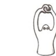
Illustrative example 2. Topological man.

By continuous deformations, a person (see picture) can unravel his fingers - a fact. It's not immediately obvious, but you can guess. But if our topological man had the foresight to put a watch on one hand, then our task will become impossible.

Let's be clear

So, I hope a couple of examples brought some clarity to what is happening.
Let's try to formalize all this in a childish way.
We will assume that we are working with plasticine figures, and plasticine can stretch, compress, while gluing different points and tearing are prohibited. Homeomorphic are figures that are transformed into each other by continuous deformations described a little earlier.

A very useful case is a sphere with handles. A sphere can have 0 handles - then it’s just a sphere, maybe one - then it’s a donut (in common parlance, a “two-dimensional torus”), etc.
So why does a sphere with handles stand out among other figures? Everything is very simple - any figure is homeomorphic to a sphere with a certain number of handles. That is, in essence, we have nothing else O_o Any three-dimensional object is structured like a sphere with a certain number of handles. Be it a cup, spoon, fork (spoon=fork!), computer mouse, person.

This is a fairly meaningful theorem that has been proven. Not by us and not now. More precisely, it has been proven for a much more general situation. Let me explain: we limited ourselves to considering figures molded from plasticine and without cavities. This entails the following troubles:
1) we can’t get a non-orientable surface (Klein bottle, Möbius strip, projective plane),
2) we limit ourselves to two-dimensional surfaces (n/a: sphere - two-dimensional surface),
3) we cannot obtain surfaces, figures extending to infinity (of course, we can imagine this, but no amount of plasticine will be enough).

The Mobius strip

Klein bottle

Term network topology means a way of connecting computers into a network. You may also hear other names - network structure or network configuration (It is the same). In addition, the concept of topology includes many rules that determine the placement of computers, methods of laying cables, methods of placing connecting equipment, and much more. To date, several basic topologies have been formed and established. Of these, we can note “ tire”, “ring" And " star”.

Bus topology

Topology tire (or, as it is often called common bus or highway ) involves the use of one cable to which all workstations are connected. The common cable is used by all stations in turn. All messages sent by individual workstations are received and listened to by all other computers connected to the network. From this stream, each workstation selects messages addressed only to it.

Advantages of the bus topology:

• ease of setup;
• relative ease of installation and low cost if all workstations are located nearby;
• The failure of one or more workstations does not in any way affect the operation of the entire network.

Disadvantages of the bus topology:

• bus problems anywhere (cable break, network connector failure) lead to network inoperability;
• difficulty in troubleshooting;
• low performance – at any given time, only one computer can transmit data to the network; as the number of workstations increases, network performance decreases;
• poor scalability - to add new workstations it is necessary to replace sections of the existing bus.

It was according to the “bus” topology that local networks were built on coaxial cable. In this case, sections of coaxial cable connected by T-connectors acted as a bus. The bus was laid through all the rooms and approached each computer. The side pin of the T-connector was inserted into the connector on the network card. This is what it looked like: Now such networks are hopelessly outdated and have been replaced everywhere by “star” twisted pair cables, but equipment for coaxial cable can still be seen in some enterprises.

Ring topology

Ring is a local network topology in which workstations are connected in series to each other, forming a closed ring. Data is transferred from one workstation to another in one direction (in a circle). Each PC works as a repeater, relaying messages to the next PC, i.e. data is transferred from one computer to another as if in a relay race. If a computer receives data intended for another computer, it transmits it further along the ring; otherwise, it is not transmitted further.

Advantages of ring topology:

• ease of installation;
• almost complete absence of additional equipment;
• Possibility of stable operation without a significant drop in data transfer speed under heavy network load.

However, the “ring” also has significant disadvantages:

• each workstation must actively participate in the transfer of information; if at least one of them fails or the cable breaks, the operation of the entire network stops;
• connecting a new workstation requires a short-term shutdown of the network, since the ring must be open during installation of a new PC;
• complexity of configuration and setup;
• Difficulty in troubleshooting.

Ring network topology is used quite rarely. It found its main application in fiber optic networks Token Ring standard.

Star topology

Star is a local network topology where each workstation is connected to a central device (switch or router). The central device controls the movement of packets in the network. Each computer is connected via a network card to the switch with a separate cable. If necessary, you can combine several networks together with a star topology - as a result you will get a network configuration with tree-like topology. Tree topology is common in large companies. We will not consider it in detail in this article.

The “star” topology today has become the main one in the construction of local networks. This happened due to its many advantages:

• failure of one workstation or damage to its cable does not affect the operation of the entire network;
• excellent scalability: to connect a new workstation, just lay a separate cable from the switch;
• easy troubleshooting and network interruptions;
• high performance;
• ease of setup and administration;
• Additional equipment can be easily integrated into the network.

However, like any topology, the “star” is not without its drawbacks:

• failure of the central switch will result in the inoperability of the entire network;
• additional costs for network equipment - a device to which all computers on the network will be connected (switch);
• the number of workstations is limited by the number of ports in the central switch.

Star – the most common topology for wired and wireless networks. An example of a star topology is a network with a twisted pair cable and a switch as the central device. These are the networks found in most organizations.

Related.
Content
General topology
Uniform topology
Algebraic topology
Piecewise linear topology
Topology of manifolds
Main stages of topology development

1. General topology
The part of theory that is oriented towards the axiomatic study of continuity is called general theory. Along with algebra, general theory forms the basis of the modern set-theoretic method in mathematics.
Axiomatically, continuity can be defined in many (generally speaking, unequal) ways. A generally accepted axiomatics is based on the concept of an open set. A topological structure, or topology, on a set X is a family of its subsets, called open sets, such that:
1) the empty set ∅ and all X are open;
2) the union of any number and the intersection of a finite number of open sets is open.
A set on which a topological structure is given is called a topological space. In the topological space X one can define all the basic concepts of elementary analysis related to continuity. For example, a neighborhood of point x
∈ X is an arbitrary open set containing this point; a set A⊂X is said to be closed if its complement XA is open; the closure of a set A is the smallest closed set containing A; if this closure coincides with X, then A is said to be everywhere dense in X, etc.
By definition, ∅ and X are both closed and open sets. If there are no other sets in X that are both closed and open, then the topological space X is called connected. A visually connected space consists of one “piece”, while an incoherent space consists of several.
Any subset A of a topological space X has a natural topological structure consisting of intersections with A of open sets from X. Equipped with this structure A is called a subspace of the space X. Each metric space becomes topological if its open sets are taken to be sets containing, together with an arbitrary point, some its ε-neighborhood (a ball of radius ε centered at this point). In particular, any subset of the n-dimensional Euclidean space |R n is a topological space. The theory of such spaces (under the name “geometric theory”) and the theory of metric spaces are traditionally included in general theory.
Geometric theory quite clearly breaks down into two parts: the study of subsets |R n of arbitrary complexity, subject to certain general restrictions (an example is the so-called theory of continua, that is, connected bounded closed sets), and the study of the ways in which |R n simple topological spaces such as sphere, ball, etc. can be embedded. (embeddings in |R n , for example, spheres, can be very complex).
An open covering of a topological space X is a family of its open sets, the union of which is the whole of X. A topological space X is called compact (in another terminology, bicompact) if any of its open coverings contains a finite number of elements forming the covering. The classical Heine-Borel theorem states that any bounded closed subset |R n is compact. It turns out that all the basic theorems of elementary analysis about bounded closed sets (for example, Weierstrass’s theorem that on such a set a continuous function reaches its greatest value) are valid for any compact topological spaces. This determines the fundamental role played by compact spaces in modern mathematics (especially in connection with existence theorems). The identification of the class of compact topological spaces was one of the greatest achievements of general theory, having general mathematical significance.
An open cover (V β) is said to be inscribed in a cover (U α) if for any β there is an α such that V β ⊂ U α. A covering (V β) is said to be locally finite if each point x ∈ X has a neighborhood intersecting only with a finite number of elements of this covering.
A topological space is said to be paracompact if any open covering of it can contain a locally finite covering. The class of paracompact spaces is an example of classes of topological spaces obtained by imposing so-called compactness type conditions. This class is very wide, in particular it contains all metrizable topological spaces, that is, spaces X in which such a metric can be introduced
ρ that the T. generated by ρ in X coincides with the T. defined in X.
The multiplicity of an open covering is the largest number k such that there are k of its elements having a non-empty intersection. The smallest number n with the property that any finite open cover of a topological space X can contain an open cover of multiplicity ≤n + 1 is denoted by dimX and is called the dimension of X.
This name is justified by the fact that in elementary geometric situations dimX coincides with the usually understood dimension, for example dim|R n = n. Other numerical functions of the topological space X are also possible, differing from dimX, but in the simplest cases coinciding with dimX. Their study is the subject of the general theory of dimension - the most geometrically oriented part of the general T. Only within the framework of this theory is it possible, for example, to give a clear and fairly general definition of the intuitive concept of a geometric figure and, in particular, the concept of a line, surface, etc.
Important classes of topological spaces are obtained by imposing the so-called separation axioms. An example is the so-called Hausdorff axiom, or T 2 axiom, which requires that any two distinct points have disjoint neighborhoods. A topological space that satisfies this axiom is called Hausdorff, or separable. For some time in mathematical practice almost exclusively Hausdorff spaces were encountered (for example, any metric space is Hausdorff). However, the role of non-Hausdorff topological spaces in analysis and geometry is constantly growing.
Topological spaces that are subspaces of Hausdorff (bi) compact spaces are called completely regular or Tikhonov. They can also be characterized by some axiom of separability, namely: an axiom requiring that for any point x 0
∈ X and any closed set F X not containing it, there existed a continuous function g: X → equal to zero at x 0 and one on F.
Topological spaces that are open subspaces of Hausdorff compact spaces are called locally compact spaces. They are characterized (in the class of Hausdorff spaces) by the fact that each of their points has a neighborhood with compact closure (example: Euclidean space). Any such space is complemented by one point to a compact one (example: by adding one point from the plane one obtains a sphere of a complex variable, and from |R n - a sphere S n).
A mapping f: X → Y of a topological space X into a topological space Y is called a continuous mapping if for any open set V ⊂ Y the set ƒ −1 (V) is open in X. A continuous mapping is called a homeomorphism if it is one-to-one and the inverse mapping f − 1:Y
→ X is continuous. Such a mapping establishes a one-to-one correspondence between open sets of topological spaces X and Y, permutable with the operations of union and intersection of sets. Therefore, all topological properties (that is, properties formulated in terms of open sets) of these spaces are the same, and from a topological point of view, homeomorphic topological spaces (that is, spaces for which there is at least one homeomorphism X → Y)
should be considered identical (just as in Euclidean geometry figures that can be combined by movement are considered identical). For example, the circle and boundary of a square, hexagon, etc. are homeomorphic (“topologically identical”). In general, any two simple (without double points) closed lines are homeomorphic. On the contrary, a circle is not homeomorphic to a straight line (because removing a point does not violate the connectedness of the circle, but does violate the connectedness of the straight line; for the same reason, a straight line is not homeomorphic to a plane, and a circle is not homeomorphic to a figure eight).
A circle is also not homeomorphic to a plane (throw out not one, but two points).
Let (X α) be an arbitrary family of topological spaces. Consider the set X of all families of the form (x α ), where x α ∈ X α (the direct product of the sets X α). For any α, the formula p α ((x α )) = x α defines some mapping p α: X → X α (called a projection). Generally speaking, in X one can introduce many topological structures with respect to which all maps p α are continuous.
Among these structures, there is a smallest one (that is, contained in any such structure). The set X equipped with this topological structure is called the topological product of the topological spaces X α and is denoted by the symbol ΠX α (and in the case of a finite number of factors, by the symbol X 1 H... H X n). Explicitly, open sets of the space X can be described as unions of finite intersections of all sets of the form p α −1 (U α), where U α is open in X α.
The topological space X has the following remarkable property of universality, which uniquely (up to homeomorphism) characterizes it: for any family of continuous maps ƒ α: Y → X α there is a unique continuous map ƒ : Y → X for which p α ∘ƒ=ƒ α for all α. The space |R n is the topological product of n instances of the number line. One of the most important theorems of general theory is the statement that the topological product of compact topological spaces is compact.
If X is a topological space and Y is an arbitrary set, and if given a mapping p: X → Y of the space X onto the set Y (for example, if Y is a quotient set of X by some equivalence relation, and p is a natural projection mapping to each element x ∈ X its equivalence class),
then we can raise the question of introducing a topological structure into Y, with respect to which the mapping p is continuous. The most “rich” (in open sets) such structure is obtained by considering all those sets V to be open sets in Y
⊂ Y for which the set f ‑1 (V) ⊂ X is open in X. The set Y equipped with this topological structure is called the quotient space of the topological space X (with respect to p). It has the property that an arbitrary map ƒ : Y
→ Z is continuous if and only if the mapping ƒ∘p: X → Z is continuous. A continuous mapping p: X → Y is called factorial if the topological space Y is, with respect to p, the quotient space of the topological space X. The continuous mapping p: X
→ Y is called open if for any open set U ⊂ X the set p(U) is open in Y, and closed if for any closed set F ⊂ X the set p(F) is closed in Y. Both open and closed continuous maps ƒ : X
→ Y, for which ƒ(X) = Y, are factorial.
Let X be a topological space, A its subspace and ƒ : A → Y a continuous map. Assuming the topological spaces X and Y are disjoint, we introduce X in their union
∪ Y topological structure, considering as open sets the unions of open sets from X and Y. In the space X ∪ Y we introduce the smallest equivalence relation in which a ∼ ƒ(α) for any point a
∈ A. The corresponding quotient space is denoted by X ∪ f Y and is said to be obtained by gluing a topological space X to a topological space Y along A via a continuous map ƒ. This simple and intuitive operation turns out to be very important, since it allows one to obtain more complex ones from relatively simple topological spaces. If Y consists of one point, then the space X
∪ f Y is denoted by the symbol X/A and is said to be obtained from X by contracting A to a point. For example, if X is a disk and A is its boundary circle, then X/A is homeomorphic to a sphere.
2. Uniform topology
The part of theory that studies the axiomatic concept of continuity is called uniform theory. The definition of uniform continuity of numerical functions, known from analysis, is directly transferred to mappings of any metric spaces. Therefore, the axiomatics of uniform continuity are usually obtained starting from metric spaces. Two axiomatic approaches to uniform continuity are explored, based respectively on the concepts of proximity and diagonal encirclement.
Subsets A and B of a metric space X are called close (notation AδB) if for any ε > 0 there are points a∈A and b∈B, the distance between which Taking the basic properties of this relation as axioms, we arrive at the following definition: (separable) structure proximity on a set X is a relation δ on the set of all its subsets such that:
1) ∅δ̅X (the symbol δ̅ denotes the negation of the relation δ;
2)
Aδ̅B 1 and Aδ̅B 2 ⇔ Aδ(B 1 U B 2);

3) (x) δ̅ (y) ⇔ x ≠ y;

4) if AδB, then there is a set Cδ̅B such that Aδ(XC).
The set in which the proximity structure is specified is called the proximity space. A mapping from a proximity space X to a proximity space Y is said to be close continuous if the images of sets that are close in X are close in Y. The proximity spaces X and Y are called close homeomorphic (or equimorphic) if there is a one-to-one close continuous mapping
X → Y, the inverse of which is also nearby continuous (such a nearby continuous mapping is called an equimorphism). In uniform theory, equimorphic proximity spaces are considered identical. Like metric spaces, any proximity space can be turned into a (Hausdorff) topological space by considering a subset
U⊂X is open if (x)δ̅(XU) for any point x∈U. In this case, nearby continuous mappings turn out to be continuous mappings. The class of topological spaces obtained in the described way from proximity spaces coincides with the class of completely regular topological spaces. For any completely regular space X, all proximity structures on X that generate its topological structure are in one-to-one correspondence with the so-called compactifications (in other terminology, bi-compact extensions) bX - compact Hausdorff topological spaces containing X as an everywhere dense space .
The proximity structure δ corresponding to the extension bX is characterized by the fact that AδB if and only if the closures of the sets A and B intersect in bX. In particular, on any compact Hausdorff topological space X there is a unique proximity structure that generates its topological structure.
Another approach is based on the fact that uniform continuity in a metric space X can be defined in terms of the relation “points x and y are at a distance not greater than ε.” From a general point of view, a relation on X is nothing more than an arbitrary subset U of the direct product XХX. The relation “identity” is, from this point of view, a diagonal Δ ⊂ X × X, that is, a set of points of the form (x, x), x∈X. For any relation U, the inverse relation U −1 = ((x,y); (y,x) is defined
∈ U) and for any two relations U and V their composition is defined U · V = ((x,y); there exists z ∈ X such that (x, z) ∈ U, (z,y) ∈ V ). A family of relations (U) is called a (separable) uniform structure on X (and relations U are called diagonal environments) if: 1) the intersection of any two diagonal environments contains a diagonal environment; 2) each diagonal environment contains
Δ, and the intersection of all diagonal surroundings coincides with Δ; 3) together with U, the environment of the diagonal is also U −1 ; 4) for any environment of the diagonal U there is an environment of the diagonal W such that W o W
⊂ U. A set endowed with a uniform structure is called a uniform space. A mapping ƒ : X → Y of a uniform space X into a uniform space Y is called uniformly continuous if the inverse image of the mapping ƒ
Х ƒ : X Х X → Y Х Y of any environment of a diagonal V ⊂ Y Х Y contains some environment of a diagonal from X Х X. Uniform spaces X and Y are called uniformly homeomorphic if there is a one-to-one uniformly continuous mapping X
→ Y, the inverse of which is also a uniformly continuous map.
In uniform T. such uniform spaces are considered identical. Each uniform structure on X defines some proximity structure: AδB if and only if (A × B) ∩ U ≠ ∅ for any diagonal environment U ⊂ X × X.
In this case, uniformly continuous maps turn out to be nearly continuous.
3. Algebraic topology
Let each topological space X (from some class) be associated with some algebraic object h(X) (group, ring, etc.), and let each continuous map ƒ : X → Y be associated with some homomorphism h(f) : h( X)
→ h(Y) (or h(f) : h(Y) → h(X), which is the identity homomorphism when ƒ is the identity map. If h(f 1 ○ f 2) = h(f 1)
○ h(f 2) (or, respectively, h(f 1 ○ f 2) = h(f 2) ○ h(f 1), then h is said to be a functor (respectively, a cofunctor). Most algebraic T problems. is somehow related to the propagation problem: for a given continuous mapping f: A
→ Y of a subspace A ⊂ X into some topological space Y, find a continuous mapping g: X → Y coinciding on A with ƒ, that is, such that ƒ = g i, where i: A
→ X - embedding map (i(a) = a for any point a ∈ A). If such a continuous map g exists, then for any functor (cofunctor) h there exists a homomorphism (φ: h(X)
→ h(Y) (homomorphism φ: h(Y) → h(X)), such that h(f) = φ ○ h(i) (respectively h(f) = h(i) ○ φ); it will be the homomorphism φ = h(g). Therefore, the non-existence of a homomorphism
φ (for at least one functor h) implies the non-existence of the mapping g. Almost all methods of algebraic T can actually be reduced to this simple principle. For example, there is a functor h, the value of which on the ball E n is a trivial group, and on the sphere S n-1 bounding the ball is a non-trivial group. This already implies the absence of the so-called retraction - a continuous mapping p: E n
→ S n-1 , fixed on S n-1 , that is, such that the composition p·i, where i: S n‑1 → E n is an embedding map, is an identity map (if p exists, then the identity map of the group h(S n-1) will be a composition of mappings h(i) : h(S n-1)
→ h(E n) and h(p) : h(E n) → h(S n-1), which is impossible for the trivial group h(E n). However, this essentially elementary geometric and (for n = 2) visually obvious fact (physically meaning the possibility of stretching a drum on a round hoop) has not yet been proven without the use of algebraic-topological methods. Its immediate consequence is the statement that any continuous map ƒ : E n
→ E n has at least one fixed point, that is, the equation ƒ(x) = x has at least one solution in E n (if ƒ(x) ≠ x for all x ∈ E n , then, taking p(x) a point from S n-1 collinear to the points ƒ(x) and x and such that the segment with ends ƒ(x) and p(x) contains x, we obtain the retraction p: E n
→ S n-1). This fixed point theorem was one of the first theorems of algebraic theory, and then became the source of a whole series of various theorems on the existence of solutions to equations.
Generally speaking, the more complex the algebraic structure of objects h(X) is, the easier it is to establish the non-existence of a homomorphism (φ). Therefore, algebraic theories consider algebraic objects of an extremely complex nature, and the requirements of algebraic topology significantly stimulated the development of abstract algebra.
A topological space X is called a cellular space, as well as a cellular partition (or CW-complex), if it contains an increasing sequence of subspaces X 0 ⊂...
⊂ X n-1 ⊂ X n ⊂... (called the skeletons of the cellular space X), the union of which is the whole of X, and the following conditions are satisfied: 1) the set U ⊂ X is open in X if and only if for any n the set U
∩ X n is open in X n ; 2) X n is obtained from X n-1 by gluing a certain family of n-dimensional balls along their boundary (n-1)-dimensional spheres (by means of an arbitrary continuous mapping of these spheres into X n-1); 3) X 0 consists of isolated points. Thus, the structure of a cellular space consists, roughly speaking, in the fact that it is represented as a union of sets homeomorphic to open balls (these sets are called cells). In algebraic techniques, cellular spaces are studied almost exclusively, since the specificity of the problems of algebraic techniques for them is already fully manifested. Moreover, in fact, some particularly simple cellular spaces (such as Polyhedra, see below) are of interest for algebraic systems, but narrowing the class of cellular spaces, as a rule, significantly complicates the study (since many useful operations on cellular spaces are derived from the class of polyhedra).
Two continuous maps f, g: X → Y are called homotopic if they can be continuously deformed into each other, that is, if there is a family of continuous maps f t: X → Y, continuously depending on the parameter t ∈ , such that f 0 = ƒ and f 1 = g (continuous dependence on t means that the formula F(x, t) = f t (x), x ∈ X, t
∈ defines a continuous mapping F: X Х → Y; this mapping, as well as the family (f t ) is called a homotopy connecting ƒ with g). The set of all continuous mappings
X → Y decomposes into homotopy classes of mappings homotopic to each other. The set of homotopy classes of continuous mappings from X to Y is denoted by the symbol . The study of properties of homotopy relations and, in particular, sets is the subject of so-called homotopy topology (or homotopy theory). For most interesting topological spaces, the sets are finite or countable and can be explicitly computed efficiently. Topological spaces X and Y are called homotopy equivalent, or having the same homotopy type, if there exist such continuous maps ƒ:
X → Y and g: Y → X such that the continuous maps g·f: X → X and f·g: Y → Y are homotopic to the corresponding identity maps. In homotopy theory, such spaces should be considered identical (all their “homotopy invariants” coincide).
It turns out that in many cases (in particular, for cellular spaces) the solvability of the propagation problem depends only on the homotopy class of the continuous map ƒ : A → Y; more precisely, if for ƒ the propagation g: X
→ Y exists, then for any homotopy f t: A → Y (with f 0 = f) there is a distribution g t: X → Y such that g 0 = g. Therefore, instead of ƒ, we can consider its homotopy class [f] and, in accordance with this, study only homotopy invariant functors (cofunctors) h, that is, such that h(f 0) = h(f 1), if the maps f 0 and f 1 homotopic. This leads to such a close interweaving of algebraic and homotopy theory that they can be considered as a single discipline.
For any topological space Y, the formulas h(X) = and h(f) = [φ○f], where f: X 1 → X 2 and φ : X 2 → Y, define some homotopy invariant cofunctor h, which is said to be that it is represented by the topological space Y. This is a standard (and essentially the only) method for constructing homotopy invariant cofunctors. In order for the set h(X) to turn out to be, say, a group, it is necessary to choose Y accordingly, for example, to require that it be a topological group (generally speaking, this is not entirely true: it is necessary to choose some point x 0 in X and consider only continuous maps and homotopies , transforming x 0 into a group unit; this technical complication will, however, be ignored in what follows). Moreover, it is sufficient for Y to be a topological group
“in the homotopy sense,” that is, so that the axioms of associativity and the existence of an inverse element (which actually assert the coincidence of some mappings) would be satisfied only “up to homotopy.” Such topological spaces are called H-spaces. Thus, each H-space Y defines a homotopy invariant cofunctor h(X) = , whose values ​​are groups.
In a similar (“dual”) way, each topological space Y is defined by the formulas h(X) = , h(f) = [ƒ ○φ], where ƒ : X 1
→ X 2 and φ : Y → X 1 , some functor h. For h(X) to be a group, Y must have a certain algebraic structure, in some well-defined sense dual to the structure of the H-space. Topological spaces endowed with this structure are called co-N-spaces. An example of a co-H-space is the n-dimensional sphere S n (for n ≥ 1).
Thus, for any topological space X, the formula π n X = defines a certain group π n X, n ≥ 1, which is called the nth homotopy group of the space X. For n = 1, it coincides with the fundamental group. For n > 1 group
π n X is commutative. If π 1 X = (1), then X is called simply connected.
A cellular space X is called a space K(G, n) if π i (X) = 0 for i ≠ n and π n X = G; such a cellular space exists for any n ≥ 1 and any group G (commutative for n > 1) and is uniquely determined up to homotopy equivalence.
For n > 1 (and also for n = 1, if the group G is commutative), the space K(G, n) turns out to be an H-space and therefore represents a certain group H n (X; G) = . This group is called the n-dimensional cohomology group of a topological space X with the coefficient group G. It is a typical representative of a number of important cofunctors, including, for example, the K-functor KO(X) = , represented by the so-called infinite-dimensional Grassmannian BO, a group of oriented cobordisms
Ω n X, etc.
If G is a ring, then the direct sum H*(X; G) of the groups H n (X; G) is an algebra over G. Moreover, this direct sum has a very complex algebraic structure, in which (for G = Z p, where Z p is a cyclic group of order p) includes the action on H*(X; G) of some non-commutative algebra p, called the Steenrod algebra. The complexity of this structure allows, on the one hand, to develop effective (but not at all simple) methods for calculating groups H n (X; G), and, on the other hand, to establish connections between groups H n (X; G) and other homotopy invariant functors (for example , homotopy groups π n X),
which often make it possible to explicitly calculate these functors.
Historically, cohomology groups were preceded by the so-called homology groups H n (X; G), which are homotopy groups π n M(X, G) of some cellular space M(X, G), uniquely constructed from the cellular space X and the group G. Homology groups and cohomology in a certain sense are dual to each other, and their theories are essentially equivalent. However, the algebraic structure found in homology groups is less familiar (for example, these groups do not constitute an algebra, but a so-called coalgebra), and therefore cohomology groups are usually used in calculations. At the same time, in some questions homology groups turn out to be more convenient, so they are also studied. The part of algebraic theory that deals with the study (and application) of homology and cohomology groups is called homology theory.
The transfer of the results of algebraic theory to spaces more general than cellular spaces is the subject of so-called general algebraic theory. In particular, general homology theory studies the homology and cohomology groups of arbitrary topological spaces and their applications. It turns out that outside the class of compact cellular spaces, different approaches to the construction of these groups lead, generally speaking, to different results, so that for non-cellular topological spaces a whole series of different homology and cohomology groups arise. The main application of the general theory of homology is in the theory of dimension and in the theory of the so-called laws of duality (describing the relationship between the topological properties of two additional subsets of topological space), and its development was largely stimulated by the needs of these theories.
4. Piecewise linear topology
A subset P ∈ |R n is called a cone with vertex a and base B if each of its points belongs to a unique segment of the form ab, where b ∈ B. A subset X ∈ |R n is called a polyhedron if any of its points has a neighborhood in X whose closure is a cone with a compact base. A continuous mapping ƒ : X → Y of polyhedra is called piecewise linear if it is linear on the rays of each conic neighborhood of any point x ∈ X. A one-to-one piecewise linear mapping, the inverse of which is also piecewise linear, is called a piecewise linear isomorphism. The subject of piecewise linear theory is the study of polyhedra and their piecewise linear mappings. In piecewise linear theory, polyhedra are considered identical if they are piecewise linearly isomorphic.
A subset X ∈ |R n is a (compact) polyhedron if and only if it is the union of a (finite) family of convex polyhedra. Any polyhedron can be represented as a union of Simplexes intersecting only along entire faces. This representation is called polyhedron triangulation. Each triangulation is uniquely determined by its simplicial scheme, that is, the set of all its vertices, in which subsets are marked, which are sets of vertices of simplexes. Therefore, instead of polyhedra, we can only consider simplicial schemes of their triangulations. For example, using a simplicial scheme one can calculate homology and cohomology groups. This is done as follows:
a) a simplex whose vertices are ordered in a certain way is called an ordered simplex of a given triangulation (or simplicial scheme) K; formal linear combinations of ordered simplices of a given dimension n with coefficients from a given group G are called n-dimensional chains; they all naturally form a group, which is denoted by the symbol C n (K; G);
b) by eliminating the vertex with number i, 0 ≤ i ≤ n, from the ordered n-dimensional simplex σ, we obtain an ordered (n-1)-dimensional simplex, which is denoted by the symbol σ (i); chain
∂σ = σ (0) −σ (1) + ... +(−1) n σ (n) is called the boundary of σ; by linearity the mapping ∂ extends to the homomorphism ∂ : C n (K; G) → C n-1 (K; G);
c) chains c for which ∂c = 0 are called cycles; they form a group of cycles Z n (K; G);
d) chains of the form ∂c are called boundaries; they constitute the group of boundaries B n (K; G);
e) it is proved that B n (K; G) ⊂ Z n (K; G) (the boundary is a cycle); therefore the factor group is defined
H n (K; G) = Z n (K; G)/ B n (K; G).
It turns out that the group H n (K; G) is isomorphic to the homology group H n (X; G) of the polyhedron X, the triangulation of which is K. A similar construction, in which one starts not from chains, but from cochains (arbitrary functions defined on the set of all ordered simplices and taking values ​​in G), gives cohomology groups.
With this construction, presented in a slightly modified form, the formation of algebraic T essentially began. In the original construction, the so-called oriented simplices (classes of ordered simplices distinguished by even permutations of vertices) were considered. This design has been developed and generalized in a wide variety of directions. In particular, its algebraic aspects gave rise to the so-called homological algebra.
In the most general way, a simplicial scheme can be defined as a set in which certain finite subsets (“simplices”) are marked, and it is required that any subset of a simplex be again a simplex. Such a simplicial scheme is a simplicial scheme for the triangulation of some polyhedron if and only if the number of elements of an arbitrary marked subset does not exceed some fixed number. However, the concept of a polyhedron can be generalized (having obtained the so-called “infinite-dimensional polyhedra”),
and then any simplicial scheme will be a triangulation scheme of some polyhedron (called its geometric realization).
An arbitrary open covering (U α ) of each topological space X can be associated with a simplicial scheme whose vertices are the elements U α of the covering and a subset of which is marked if and only if the elements of the covering constituting this subset have a non-empty intersection. This simplicial diagram (and the corresponding polyhedron) is called a covering nerve. The nerves of all possible coverings in a certain sense approximate the space X and, based on their homology and cohomology groups, it is possible, by means of an appropriate passage to the limit, to obtain the homology and cohomology groups of X itself. This idea underlies almost all constructions of the general theory of homology. The approximation of topological space by the nerves of its open coverings also plays an important role in general T.
5. Topology of manifolds
A Hausdorff paracompact topological space is called an n-dimensional topological manifold if it is “locally Euclidean,” that is, if each of its points has a neighborhood (called a coordinate neighborhood, or map) homeomorphic to the topological space |Rn. In this neighborhood, points are specified by n numbers x 1,
..., x n, called local coordinates. At the intersection of two maps, the corresponding local coordinates are expressed in terms of each other through certain functions called transition functions. These functions define a homeomorphism of open sets in |R n and are called a transition homeomorphism.
Let us agree to call an arbitrary homeomorphism between open sets in |R n a t-homeomorphism. A homeomorphism that is a piecewise linear isomorphism will be called a p-homeomorphism, and if it is expressed by smooth (differentiable any number of times) functions, we will call it an s-homeomorphism.
Let α = t, p or s. A topological manifold is called an α-manifold if its coverage with maps is chosen such that the transition homeomorphisms for any two of its (intersecting) maps are α-homeomorphisms. Such a covering defines an α-structure on the topological manifold X.
So a t-manifold is just any topological manifold, p-manifolds are called piecewise linear manifolds. Every piecewise linear manifold is a polyhedron. In the class of all polyhedra, n-dimensional piecewise linear manifolds are characterized by the fact that any of their points has a neighborhood piecewise linearly isomorphic to the n-dimensional cube. s-manifolds are called smooth (or differentiable) manifolds. An α-map is an α-manifold that is called an arbitrary continuous mapping for α = t, an arbitrary piecewise linear mapping for α = s, an arbitrary smooth mapping for α = s, that is, a continuous mapping written in local coordinates by smooth functions.
A one-to-one α-map, the inverse of which is also an α-map, is called an α-homeomorphism (for α = s, also a diffeomorphism), α-manifolds X and Y are called α-homeomorphic (for α = s, diffeomorphic) if there exists although would be one
α-homeomorphism X → Y.
The subject of the theory of α-manifolds is the study of α-manifolds and their α-mappings; in this case, α-homeomorphic α-manifolds are considered identical. The theory of s-manifolds is part of piecewise linear T. The theory of s-manifolds is also called smooth T.
The main method of modern manifold theory is to reduce its problems to problems of algebraic theory for certain appropriately constructed topological spaces. This close connection between the theory of varieties and algebraic theory made it possible, on the one hand, to solve many difficult geometric problems, and on the other hand, it sharply stimulated the development of algebraic theory itself.
Examples of smooth manifolds are n-dimensional surfaces in |R n that do not have singular points. It turns out (embedding theorem) that any smooth manifold is diffeomorphic to such a surface (for N ≥ 2n + 1). A similar result is also true for α = t, p.
Every p-variety is a t-variety. It turns out that on any s-manifold one can introduce a p-structure in a natural way (which is usually called Aithead triangulation). We can say that any α-manifold where α = p or s is an α’-manifold where α’ = t or p.
The answer to the opposite question: on which α’-manifolds can we introduce an α-structure (such an α’-manifold with α’ = p is called smooth, and with α’ = t - triangulated),
and if possible, then how much? - depends on the dimension n.
There are only two one-dimensional topological manifolds: the circle S 1 (compact manifold) and the straight line |R (non-compact manifold). For any α = p, s there is a unique α-structure on the t-manifolds S 1 and |R.
Similarly, on any two-dimensional topological manifold (surface) there is a unique α-structure, and all compact connected surfaces can be easily described (non-compact connected surfaces can also be described, but the answer is more complex). For surfaces to be homeomorphic, it is sufficient that they are homotopy equivalent. Moreover, the homotopy type of any surface is uniquely characterized by its homology groups. There are two types of surfaces: orientable and non-orientable. Among the orientables are the sphere SI and the torus TI. Let X and Y be two connected n-dimensional α-manifolds.
Let's cut out a ball in X and Y (for n = 2 - a disk) and glue the resulting boundary spheres (for n = 2 - circles). Subject to some self-evident precautions, the result is again an α-manifold.
It is called the connected sum of α-manifolds X and Y and is denoted by X#Y. For example, TI#TI has the shape of a pretzel. The sphere S n is the zero of this addition, that is, S n #X = X for any X. In particular, SІ#TI = TI. It turns out that the orientable surface is homeomorphic to a connected sum of the form SІ#TI#
...#TI, the number p of terms TI is called the genus of the surface. For a sphere p = 0, for a torus p = 1, etc. A surface of genus p can be visualized as a sphere to which p “handles” are glued.
Every non-orientable surface is homeomorphic to a connected sum |RPI#... #|RPI of a certain number of projective planes |RPI. It can be imagined as a sphere to which several Mobius sheets are glued.
On every three-dimensional topological manifold for any α = p, s there is also a unique α-structure and it is possible to describe all homotopy types of three-dimensional topological manifolds (however, homology groups are no longer sufficient for this). At the same time, until now (1976) all (at least compact connected) Poincaré conjectures have not been described, it is unknown.
It is remarkable that for compact and connected topological varieties of dimension n ≥ 5 the situation turns out to be completely different: all the main problems for them can be considered solved in principle (more precisely, reduced to problems of algebraic theory). Any smooth manifold X is embedded as a smooth (n-dimensional) surface in IR N and the tangent vectors to X constitute some new smooth manifold TX, which is called the tangent bundle of a smooth manifold X. In general, a vector bundle over a topological space X is called a topological space E, for which is given such a continuous mapping
π : E → X such that for every point x ∈ X the inverse image of v (layer) is a vector space and there is an open covering (U α ) of the space X such that for any α the inverse image
π −1 (U α) is homeomorphic to the product U α × |R n , and there is a homeomorphism π −1 (U α) → U α × |R n , linearly mapping each layer
π −1 (x), x ∈ U α, to the vector space (x) H |R n. When E = TX, the continuous map π associates with each tangent vector the point of its tangency, so that the layer
π −1 (x) will be the space tangent to X at point x. It turns out that any vector bundle over a compact space X defines some element of the group KO(X). Thus, in particular, for any smooth, compact and connected manifold X in the group KO(X) there is defined an element corresponding to the tangent bundle. It is called the tangential invariant of a smooth variety X. There is an analogue of this construction for any α.
For α = p, the role of the group KO(X) is played by some other group, denoted KPL(X), and for α = t, the role of this group is played by a group denoted KTop(X). Each α-manifold X defines in the corresponding group [KO(X), KPL(X) or KTop(X)] some element called its α-tangential invariant.
There are natural homomorphisms KO(X) → KPL(X) → KTop(X), and it turns out that on an n-dimensional (n ≥ 5) compact and connected α-manifold X, where α = t, p, if and only if one can introduce an α-structure (α = p if α = t, and α = s if α = p) when its α-tangential invariant lies in the image of the corresponding group.
The number of such structures is finite and equal to the number of elements of some factor set of the set , where Y α is some specially constructed topological space (for α = s, the topological space Y α is usually denoted by the symbol PL/O, and for α = p - by the symbol Top/PL).
Thus, the question of the existence and uniqueness of an α-structure is reduced to a certain problem in homotopy theory. The homotopy type of the topological space PL/O is quite complicated and has not yet been completely calculated (1976); however, it is known that
π i (PL/O) = 0 for i ≤ 6, it follows that any piecewise linear manifold of dimension n ≤ 7 is smoothable, and for n ≤ 6 in a unique way. On the contrary, the homotopy type of the topological space Top/PL turns out to be surprisingly simple: this space is homotopy equivalent to K(ℤ 2 , 3).
Consequently, the number of piecewise linear structures on a topological manifold does not exceed the number of elements of the group H i(X, ℤ 2). Such structures certainly exist if H 4 (X, ℤ 2)
= 0, but for H 4 (X, ℤ 2) ≠ 0 the piecewise linear structure may not exist.
In particular, there is a unique piecewise linear structure on the sphere S n. There can be many smooth structures on the sphere S n, for example, on S 7 there are 28 different smooth structures. On the torus T n (the topological product of n copies of the circle S 1) there exist for n ≥ 5 many different piecewise linear structures, which all admit a smooth structure.
Thus, the first one is equivalent to the sphere and is homeomorphic to it).
Along with α-manifolds, we can consider the so-called α-manifolds with boundary; they are characterized by the fact that the neighborhoods of some of their points (constituting the edge) are α-homeomorphic to the half-space X n ≥ 0 of the space |R n . A boundary is an (n-1)-dimensional α-manifold (generally speaking, disconnected).
Two n-dimensional compact α-manifolds X and Y are said to be (co)bordant if there exists an (n+1)-dimensional compact α-manifold with boundary W such that its boundary is the union of disjoint smooth varieties α-homeomorphic to X and Y .
If the embedding maps X → W and Y → W are homotopy equivalences, then the smooth manifolds are called h-cobordant. Using handle decomposition methods, it is possible to prove that for n ≥ 5 simply connected compact α-manifolds are α-homeomorphic if they are h-cobordant.
This h-cobordism theorem provides the strongest way to establish the α-homeomorphy of α-manifolds (in particular, the Poincaré conjecture is a corollary of it). A similar but more complex result also holds for non-simply connected α-manifolds.
The collection of n classes of cobordant compact α-manifolds is a commutative group with respect to the connected sum operation. The zero of this group is the class of α-manifolds that are edges, that is, cobordant to zero. It turns out that this group for α = s is isomorphic to the homotopy group π 2n+1 MO (n+1) of some specially constructed topological space MO (n+1), called the Thom space.
A similar result occurs for α = p, t. Therefore, the methods of algebraic theory make it possible, in principle, to calculate the group α n. In particular, it turns out that the group s n is a direct sum of groups ℤ 2 in an amount equal to the number of partitions of the number n into terms other than numbers of the form 2 m -1. For example, s 3 = 0 (so every three-dimensional compact smooth manifold is a boundary).
On the contrary, s 2 = ℤ 2, so there are surfaces that are cobordant to each other and not cobordant to zero; such a surface, for example, is the projective plane |RP I.
M. M. Postnikov.
6. Main stages of topology development
Some results of a topological nature were obtained back in the 18th and 19th centuries. (Euler’s theorem on convex polyhedra, classification of surfaces and Jordan’s theorem that a simple closed line lying in a plane splits the plane into two parts). At the beginning of the 20th century. a general concept of space in space is created (metric - M. Fréchet, topological - F. Hausdorff), and a (bi)compact extension of a completely regular space is built under the influence of Elements; homology groups of arbitrary spaces are defined (Cech), into cohomology groups (J. homotopy theory (H. Hopf, Pontryagin); homotopy groups are defined (V. in France, M. M. Postnikov in the USSR, Whitehead, etc.) the theory is finally formed homotopies. At this time, large centers of algebraic topology were created in the USA, and triangulability (J. Milnor, USA). A, Differential Topology. Beginning Course, translated from English, Moscow, 1972; Steenrod N., Chinn W. , First concepts of topology, translated from English, M., 1967; Alexandrov P. S., Combinatorial topology, M.-L., 1947; Alexandrov P. S., Pasynkov B. A., Introduction to the theory of dimension.
Introduction to the theory of topological spaces and the general theory of dimension, M., 1973; Aleksandrov P.S., Introduction to the homological theory of dimension and general combinatorial topology, M., 1975; Arkhangelsky A.V., Ponomarev V.I., Fundamentals of general topology in problems and exercises, M., 1974; Postnikov M. M., Introduction to Morse theory, M., 1971; Bourbaki N., General topology. Basic structures, trans. from French, M., 1968; his, General topology. Topological groups. Numbers and related groups and spaces, trans. from French, M., 1969; his, General topology.

A computer network can be divided into two components. A physical computer network is, first of all, equipment. That is, all the required cables and adapters connected to computers, hubs, switches, printers, and so on. Everything that should work on a common network.

The second component of a computer network is the logical network. This is the principle of connecting a number of computers and the necessary equipment into a single system (the so-called computer network topology). This concept is more applicable to local networks. It is the selected topology for connecting a number of computers that will influence the required equipment, the reliability of the network, the possibility of its expansion, and the cost of work. Nowadays, the most widely used types of computer network topologies are ring, star, and bus. The latter, however, has almost gone out of use.

Star, ring, and bus are the basic topologies of computer networks.

"Star"

The topology of computer networks “star” is a structure whose center is a switching device. All computers are connected to it via separate lines.

The switching device can be a hub, that is, a HUB, or a switch. This topology is also called “passive star”. If the switching device is another computer or server, then the topology may be called an “active star”. It is the switching device that receives the signal from each computer, is processed and sent to other connected computers.

This topology has a number of advantages. The undoubted advantage is that the computers do not depend on each other. If one of them breaks down, the network itself remains in working order. You can also easily connect a new computer to such a network. When new equipment is connected, the remaining elements of the network will continue to operate as usual. In this type of network topology it is easy to find faults. Perhaps one of the main advantages of the “star” is its high performance.

However, despite all the advantages, this type of computer network also has disadvantages. If the central switching device fails, the entire network will stop working. It has restrictions on connected workstations. There cannot be more than the available number of ports on the switching device. And the last disadvantage of the network is its cost. A fairly large amount of cable is required to connect each computer.

"Ring"

The topology of computer networks “ring” does not have a structural center. Here, all workstations together with the server are united in a closed circle. In this system, the signal moves sequentially from right to left in a circle. All computers are repeaters, so the marker signal is maintained and transmitted further until it reaches the recipient.

This type of topology also has both advantages and disadvantages. The main advantage is that the operation of the computer network remains stable even under heavy load. This type of network is very easy to install and requires a minimal amount of additional equipment.

Unlike the “star” topology, in the “ring” topology the operation of the entire system can be paralyzed by the failure of any connected computer. Moreover, identifying the malfunction will be much more difficult. Despite the easy installation of this network option, its configuration is quite complex and requires certain skills. Another disadvantage of this topology is the need to suspend the entire network to connect new equipment.

"Tire"

The bus topology of computer networks is now becoming less and less common. It consists of a single long backbone to which all computers are connected.

In this system, as in others, the data is sent along with the recipient's address. All computers receive the signal, but it is received directly by the recipient. Workstations connected by a bus topology cannot send data packets at the same time. While one of the computers performs this action, the others wait their turn. The signals move along the line in both directions, but when they reach the end, they are reflected and overlap each other, threatening the smooth operation of the entire system. There are special devices - terminators designed to dampen signals. They are installed at the ends of the highway.

The advantages of the “bus” topology include the fact that such a network can be installed and configured quite quickly. In addition, its installation will be quite cheap. If one of the computers fails, the network will continue to operate as usual. Connecting new equipment can be done in working order. The network will function.

If the central cable is damaged or one of the terminators stops working, this will lead to a shutdown of the entire network. Finding a fault in such a topology is quite difficult. An increase in the number of workstations reduces network performance and also leads to delays in information transfer.

Derived computer network topologies

The classification of computer networks by topology is not limited to three basic options. There are also such types of topologies as “line”, “double ring”, “mesh topology”, “tree”, “lattice”, “close network”, “snowflake”, “fully connected topology”. All of them are derived from the basic ones. Let's look at some options.

Inefficient topologies

In a mesh topology, all workstations are connected to each other. Such a system is quite cumbersome and ineffective. It is required to allocate a line for each pair of computers. This topology is used only in multi-machine systems.

The mesh topology is, in fact, a stripped-down version of the fully connected one. Here, too, all computers are connected to each other via separate lines.

Most efficient topologies

The topology for building computer networks called “snowflake” is a stripped-down version of the “star”. Here, hubs connected to each other in a star-type act as workstations. This topology option is considered one of the most optimal for large local and global networks.

As a rule, large local as well as global networks have a huge number of subnets built on different types of topologies. This type is called mixed. Here you can simultaneously distinguish the “star”, the “tire”, and the “ring”.

So, in the above article, all the main available computer network topologies used in local and global networks, their variations, advantages and disadvantages were considered.

Explanatory dictionary of the Russian language. D.N. Ushakov

topology

topology, many no, w. (from Greek topos - place and logos - teaching) (mat.). Part of geometry that studies the qualitative properties of figures (i.e., independent of concepts such as length, angles, straightness, etc.).

New explanatory dictionary of the Russian language, T. F. Efremova.

topology

and. A branch of mathematics that studies the qualitative properties of geometric figures, independent of their length, angles, straightness, etc.

Encyclopedic Dictionary, 1998

topology

TOPOLOGY (from the Greek topos - place and... logic) is a branch of mathematics that studies the topological properties of figures, i.e. properties that do not change under any deformations produced without breaks and gluing (more precisely, with one-to-one and continuous mappings). Examples of topological properties of figures are dimension, the number of curves bounding a given area, etc. Thus, a circle, an ellipse, and the outline of a square have the same topological properties, because these lines can be deformed into one another in the manner described above; at the same time, the ring and the circle have different topological properties: the circle is limited by one contour, and the ring by two.

Topology

(from the Greek topos ≈ place and ¼ logy) ≈ part of geometry devoted to the study of the phenomenon of continuity (expressed, for example, in the concept of limit). The variety of manifestations of continuity in mathematics and a wide range of different approaches to its study led to the disintegration of unified mathematics into a number of departments (“general mathematics,” “algebraic mathematics,” etc.), differing from each other in subject and method of study and in fact very little related to each other. I. General topology The part of theory that is oriented towards the axiomatic study of continuity is called general theory. Along with algebra, general theory forms the basis of the modern set-theoretic method in mathematics. Axiomatically, continuity can be defined in many (generally speaking, unequal) ways. A generally accepted axiomatics is based on the concept of an open set. A topological structure, or topology, on a set X is a family of its subsets, called open sets, such that: 1) the empty set Æ and all X are open; 2) the union of any number and the intersection of a finite number of open sets is open. A set on which a topological structure is given is called a topological space. In the topological space X one can define all the basic concepts of elementary analysis related to continuity. For example, a neighborhood of a point x О X is an arbitrary open set containing this point; a set A Ì X is called closed if its complement X \ A is open; the closure of a set A is the smallest closed set containing A; if this closure coincides with X, then A is said to be everywhere dense in X, etc. By definition, Æ and X are both closed and open sets. If there are no other sets in X that are both closed and open, then the topological space X is called connected. A visually connected space consists of one “piece,” while a disconnected space consists of several. Any subset A of a topological space X has a natural topological structure consisting of intersections with A of open sets from X. Equipped with this structure A is called a subspace of the space X. Each metric space becomes topological if its open sets are taken to be sets containing, together with an arbitrary point, some its e-neighborhood (a ball of radius e centered at this point). In particular, any subset of an n-dimensional Euclidean space ═is a topological space. The theory of such spaces (under the name “geometric theory”) and the theory of metric spaces are traditionally included in general theory. Geometric theory is quite clearly divided into two parts: the study of subsets of arbitrary complexity, subject to certain restrictions of a general nature (an example is the so-called theory of continua, that is, connected bounded closed sets), and the study of the ways in which such simple topological spaces as a sphere, ball, etc. can be embedded in ═. (investments in, for example, spheres can be very complex). An open covering of a topological space X is a family of its open sets, the union of which is the whole of X. A topological space X is called compact (in other terminology, bicompact) if any of its open coverings contains a finite number of elements that also form the covering. The classical Heine ≈ Borel theorem states that any bounded closed subset is ═compact. It turns out that all the basic theorems of elementary analysis about bounded closed sets (for example, Weierstrass’s theorem that on such a set a continuous function reaches its greatest value) are valid for any compact topological spaces. This determines the fundamental role played by compact spaces in modern mathematics (especially in connection with existence theorems). The identification of the class of compact topological spaces was one of the greatest achievements of general theory, having general mathematical significance. An open cover (Vb) is said to be inscribed in a cover (Ua) if for any b there exists an a such that Vb Ì Ua. A covering (Vb) is called locally finite if each point x Î X has a neighborhood intersecting only with a finite number of elements of this covering. A topological space is said to be paracompact if any open covering of it can contain a locally finite covering. The class of paracompact spaces is an example of classes of topological spaces obtained by imposing so-called compactness type conditions. This class is very wide; in particular, it contains all metrizable topological spaces, that is, spaces X in which it is possible to introduce a metric r such that the T generated by r in X coincides with the T defined in X. The multiplicity of an open covering is the largest the number k is such that there are k of its elements having a non-empty intersection. The smallest number n, which has the property that an open cover of multiplicity £n + 1 can be inscribed into any finite open cover of a topological space X, is denoted by the symbol dimX and is called the dimension of X. This name is justified by the fact that in elementary geometric situations dimX coincides with the usual understandable dimension, for example dim = n. Other numerical functions of the topological space X are also possible, differing from dimX, but in the simplest cases coinciding with dimX. Their study is the subject of the general theory of dimension, the most geometrically oriented part of the general T. Only within the framework of this theory is it possible, for example, to give a clear and fairly general definition of the intuitive concept of a geometric figure and, in particular, the concept of a line, surface, etc. Important classes of topological spaces are obtained by imposing the so-called separation axioms. An example is the so-called Hausdorff axiom, or axiom T2, which requires that any two distinct points have disjoint neighborhoods. A topological space that satisfies this axiom is called Hausdorff, or separable. For some time in mathematical practice almost exclusively Hausdorff spaces were encountered (for example, any metric space is Hausdorff). However, the role of non-Hausdorff topological spaces in analysis and geometry is constantly growing. Topological spaces that are subspaces of Hausdorff (bi) compact spaces are called completely regular or Tikhonov. They can also be characterized by some axiom of separability, namely: an axiom requiring that for any point x0 ═X and any closed set F ═X not containing it, there exists a continuous function g: X ╝ equal to zero at x0 and one on F. Topological spaces that are open subspaces of Hausdorff compact spaces are called locally compact spaces. They are characterized (in the class of Hausdorff spaces) by the fact that each of their points has a neighborhood with compact closure (example: Euclidean space). Any such space is complemented by one point to a compact one (example: by adding one point from the plane one obtains a sphere of a complex variable, and from ═≈ a sphere S n). A mapping f: X ╝ Y from a topological space X to a topological space Y is called a continuous mapping if for any open set V М Y the set f≈1(V) is open in X. A continuous mapping is called a homeomorphism if it is one-to-one and the inverse mapping f≈ 1: Y ╝ X continuous. Such a mapping establishes a one-to-one correspondence between open sets of topological spaces X and Y, permutable with the operations of union and intersection of sets. Therefore, all topological properties (that is, properties formulated in terms of open sets) of these spaces are the same, and from a topological point of view, homeomorphic topological spaces (that is, spaces for which there is at least one homeomorphism X ╝ Y) should be considered the same ( just as in Euclidean geometry figures that can be combined by movement are considered identical). For example, the circle and boundary of a square, hexagon, etc. are homeomorphic (“topologically identical”). In general, any two simple (without double points) closed lines are homeomorphic. On the contrary, a circle is not homeomorphic to a straight line (because removing a point does not violate the connectedness of the circle, but does violate the connectedness of the straight line; for the same reason, a straight line is not homeomorphic to a plane, and a circle is not homeomorphic to a figure eight). A circle is also not homeomorphic to a plane (throw out not one, but two points). Let (Xa) ≈ an arbitrary family of topological spaces. Consider the set X of all families of the form (xa), where xa ═Xa (the direct product of the sets Xa). For any a, the formula defines some mapping ═ (called a projection). Generally speaking, in X one can introduce many topological structures with respect to which all maps pa are continuous. Among these structures, there is a smallest one (that is, contained in any such structure). The set X equipped with this topological structure is called the topological product of topological spaces Xa and is denoted by the symbol PHa (and in the case of a finite number of factors, by the symbol X1 ` ... ` Xn). Explicitly, open sets of the space X can be described as unions of finite intersections of all sets of the form where Ua is open in Xa. The topological space X has the following remarkable property of universality, which uniquely (up to homeomorphism) characterizes it: for any family of continuous mappings fa: Y ╝ Xa there is a unique continuous mapping f: Y ╝ X for which ══for all a. The space ═is the topological product of n instances of the number line. One of the most important theorems of general theory is the statement that the topological product of compact topological spaces is compact. If X ≈ topological space, and Y ≈ an arbitrary set, and if a mapping p: X ╝ Y of the space X onto the set Y is given (for example, if Y is a quotient set of X by some equivalence relation, and p is a natural projection mapping to each element x Î X is its equivalence class), then we can raise the question of introducing into Y a topological structure with respect to which the mapping p is continuous. The most “rich” (in open sets) such structure is obtained by considering as open sets in Y all those sets V Ì Y for which the set f‑1(V) Ì X is open in X. The set Y equipped with this topological structure is called the quotient space of the topological space X (relative to p). It has the property that an arbitrary mapping f: Y ╝ Z is continuous if and only if the mapping ═: X ╝ Z is continuous. A continuous mapping p: X ╝ Y is called factor if the topological space Y is a factor space of the topological space with respect to p X. A continuous mapping p: X ╝ Y is called open if for any open set U Ì X the set p(U) is open in Y, and closed if for any closed set F Ì X the set p(F) is closed in Y. How open and closed continuous maps f: X ╝ Y for which f(X) = Y are factorial. Let X ≈ a topological space, A ≈ its subspace, and f: A ╝ Y ≈ a continuous map. Assuming the topological spaces X and Y are disjoint, we introduce a topological structure in their union X È Y, considering the unions of open sets from X and Y to be open sets. Next, we introduce in the space X È Y the smallest equivalence relation in which a ~ f(a) for any point a Î A. The corresponding quotient space is denoted by the symbol X È fY, and it is said to be obtained by gluing the topological space X to the topological space Y along A by means of a continuous map f. This simple and intuitive operation turns out to be very important, since it allows one to obtain more complex ones from relatively simple topological spaces. If Y consists of one point, then the space X È fY is denoted by the symbol X/A and is said to be obtained from X by contracting A to a point. For example, if X ≈ a disk, and A ≈ its boundary circle, then X/A is homeomorphic to a sphere. 2. Uniform topology The part of theory that studies the axiomatic concept of uniform continuity is called uniform theory. The definition of uniform continuity of numerical functions, known from analysis, is directly transferred to mappings of any metric spaces. Therefore, the axiomatics of uniform continuity are usually obtained starting from metric spaces. Two axiomatic approaches to uniform continuity, based respectively on the concepts of proximity and diagonal encirclement, are explored in detail. Subsets A and B of the metric space X are called close (notation AdB) if for any e > 0 there exist points a Î A and b Î B, the distance between which< e. Принимая основные свойства этого отношения за аксиомы, приходят к следующему определению: (отделимой) структурой близости на множестве Х называется такое отношение d на множестве всех его подмножеств, что: 1) ÆX (символом обозначается отрицание отношения d; 2) AB1 и AB2Û A(B1 U B2); ═3) {x}{y} Û x ¹ y;4) если АВ, то существует такое множество С В, что А(Х\С). Множество, в котором задана структура близости, называется пространством близости. Отображение пространства близости Х в пространство близости Y называется близостно непрерывным, если образы близких в Х множеств близки в Y. Пространства близости Х и Y называются близостно гомеоморфными (или эквиморфными), если существует взаимно однозначное близостно непрерывное отображение X ╝ Y, обратное к которому также является близостно непрерывным (такое близостно непрерывное отображение называется эквиморфизмом). В равномерной Т. эквиморфные пространства близости рассматриваются как одинаковые. Подобно метрическим пространствам, любое пространство близости можно превратить в (хаусдорфово) топологическое пространство, считая подмножество u Ì x открытым, если {x}(X \U) для любой точки х Î U. При этом близостно непрерывные отображения окажутся непрерывными отображениями. Класс топологических пространств, получающихся описанным образом из пространств близости, совпадает с классом вполне регулярных топологических пространств. Для любого вполне регулярного пространства Х все структуры близости на X, порождающие его топологическую структуру, находятся во взаимно однозначном соответствии с так называемыми компактификациями (в другой терминологии ≈ би-компактными расширениями) вХ ≈ компактными хаусдорфовыми топологическими пространствами, содержащими Х в качестве всюду плотного пространства. Структура близости d, соответствующая расширению вХ, характеризуется тем, что АdВ тогда и только тогда, когда замыкания множеств А и В пересекаются в bX. В частности, на любом компактном хаусдорфовом топологическом пространстве Х существует единственная структура близости, порождающая его топологическую структуру. Другой подход основан на том, что равномерную непрерывность в метрическом пространстве Х можно определить в терминах отношения «точки х и у находятся на расстоянии, не большем e». С общей точки зрения, отношение на Х есть не что иное как произвольное подмножество U прямого произведения Х ` X. Отношение «тождество» является с этой точки зрения диагональю D Ì Х ` X, то есть множеством точек вида (х, х), х Î X. Для любого отношения U определено обратное отношение U≈1 = {(х, у); (у, х) Î U } и для любых двух отношений U и V определена их композиция U × V = {(х, у); существует z Î Х такое, что (х, z) Î U, (z, y) Î V }. Семейство отношений {U } называется (отделимой) равномерной структурой на Х (а отношения U называется окружениями диагонали), если: 1) пересечение любых двух окружений диагонали содержит окружение диагонали; 2) каждое окружение диагонали содержит D, и пересечение всех окружений диагонали совпадает с D; 3) вместе с U окружением диагонали является и U≈1; 4) для любого окружения диагонали U существует такое окружение диагонали W, что W o W Ì U. Множество, наделённое равномерной структурой, называется равномерным пространством. Отображение f: X ╝ Y равномерного пространства Х в равномерное пространство Y называется равномерно непрерывным, если прообраз при отображении f ` f: Х ` Х ╝ Y ` Y любого окружения диагонали V Ì Y ` Y содержит некоторое окружение диагонали из Х ` X. Равномерные пространства Х и Y называются равномерно гомеоморфными, если существует взаимно однозначное равномерно непрерывное отображение Х ╝ Y, обратное к которому также является равномерно непрерывным отображением. В равномерной Т. такие равномерные пространства считаются одинаковыми. Каждая равномерная структура на Х определяет некоторую структуру близости: АdВ тогда и только тогда, когда (A ` В) Ç U ¹ Æ для любого окружения диагонали U Ì X ` X. При этом равномерно непрерывные отображения оказываются близостно непрерывными. 3. Algebraic topology Let each topological space X (from some class) be associated with some algebraic object h(X) (group, ring, etc.), and let each continuous mapping f: X ╝ Y ≈ some homomorphism h(f) : h( X) ╝ h(Y) (or h(f) : h(Y) ╝ h(X), which is the identity homomorphism when f is the identity map. If h(f1 ═f2) = h(f1) ═h( f2) (or, respectively, h(f1 ═f2) = h(f2) h(f1), then we say that h is a functor (respectively, a cofunctor). Most problems in algebraic theory are in one way or another related to the following propagation problem: for a given continuous mapping f: A ╝ Y of the subspace A Ì X into some topological space Y, find a continuous mapping g: X ╝ Y coinciding on A with f, that is, such that f = g×i, where i: A ╝ X ≈ embedding mapping (i(a) = a for any point a О A). If such a continuous mapping g exists, then for any functor (cofunctor) h there exists a homomorphism (j: h(X) ╝ h(Y) (homomorphism j: h(Y) ╝ h(X)), such that h(f) = j ═h(i) (respectively, h(f) = h(i) ═j); it will be the homomorphism j = h(g). Consequently, the non-existence of a homomorphism j (at least for one functor h) implies the non-existence of the mapping g. Almost all methods of algebraic T can actually be reduced to this simple principle. For example, there is a functor h whose value on the ball E n is a trivial group, and on the sphere S n≈1 ≈ a nontrivial group bounding the ball. This already implies the absence of the so-called retraction ≈ continuous mapping р: E n╝ S n≈1, fixed on S n≈1, that is, such that the composition р×i, where i: S n‑1 ╝ E n ≈ embedding mapping , is an identity mapping (if p exists, then the identity mapping of the group h(S n≈1) will be a composition of the mappings h(i) : h(S n≈1) ╝ h(E n) and h(p) : h( E n) ╝ h(S n≈1), which is impossible for a trivial group h(E n). However, this essentially elementary geometric and (for n = 2) visually obvious fact (physically meaning the possibility of stretching a drum on a round hoop) has not yet been proven without the use of algebraic-topological methods. Its immediate consequence is the statement that any continuous mapping f: E n╝ E n has at least one fixed point, that is, the equation f(x) = x has at least one solution in E n (if f(x) ¹ x for all x О E n, then, taking p(x) to be a point from S n≈1, collinear to the points f(x) and x and such that the segment with ends f(x) and p(x) contains x, we obtain the retraction р: E n╝ S n≈1). This fixed point theorem was one of the first theorems of algebraic theory, and then became the source of a whole series of various theorems on the existence of solutions to equations. Generally speaking, establishing the non-existence of a homomorphism (j is easier, the more complex the algebraic structure of objects h(X). Therefore, in algebraic theories, algebraic objects of an extremely complex nature are considered, and the requirements of algebraic topology significantly stimulated the development of abstract algebra. The topological space X is called a cellular space, as well as a cellular partition (or CW-complex), if it contains an increasing sequence of subspaces X 0 М ¼ М X n≈1 М X n М ¼ (called the skeletons of a cellular space X), the union of which is the whole of X, and the following conditions are satisfied : 1) the set U Ì X is open in X if and only if for any n the set U Ç X n is open in X n; 2) X n is obtained from X n≈1 by gluing a certain family of n-dimensional balls along their boundary (n≈1)-dimensional spheres (by means of an arbitrary continuous mapping of these spheres to X n≈1); 3) X0 consists of isolated points. Thus, the structure of a cellular space consists, roughly speaking, in the fact that it is represented as a union of sets homeomorphic to open balls (these sets are called cells). In algebraic techniques, cellular spaces are studied almost exclusively, since the specificity of the problems of algebraic techniques for them is already fully manifested. Moreover, in fact, some particularly simple cellular spaces (such as polyhedra, see below) are of interest for algebraic theory, but narrowing the class of cellular spaces, as a rule, significantly complicates the study (since many useful operations on cellular spaces are derived from the class of polyhedra). Two continuous maps f, g: X ╝ Y are called homotopic if they can be continuously deformed into each other, that is, if there is a family of continuous maps ft: X ╝ Y that continuously depend on the parameter t О such that f0= f and f1 = g (continuous dependence on t means that the formula F(x, t) = ft(x), x О X, t О defines a continuous map F: X ` ╝ Y; this map, as well as the family (ft) is called a homotopy , connecting f to g). The set of all continuous mappings X ╝ Y splits into homotopy classes of mappings homotopic to each other. The set of homotopy classes of continuous mappings from X to Y is denoted by the symbol . The study of properties of homotopy relations and, in particular, sets is the subject of so-called homotopy topology (or homotopy theory). For most interesting topological spaces, the sets are finite or countable and can be explicitly computed efficiently. Topological spaces X and Y are called homotopy equivalent, or having the same homotopy type, if there are continuous maps f: X ╝ Y and g: Y ╝ X such that continuous maps g×f: X ╝ X and f×g: Y ╝ Y are homotopic to the corresponding identity mappings. In homotopy theory, such spaces should be considered identical (all their “homotopy invariants” coincide). It turns out that in many cases (in particular, for cellular spaces) the solvability of the propagation problem depends only on the homotopy class of the continuous mapping f: A ╝ Y; more precisely, if for f the distribution g: X ╝ Y exists, then for any homotopy ft: A ╝ Y (with f0 = f) there exists a distribution gt: X ╝ Y such that g0 = g. Therefore, instead of f, we can consider its homotopy class [f] and, in accordance with this, study only homotopy invariant functors (cofunctors) h, that is, such that h(f0) = h(f1) if the maps f0 and f1 are homotopic. This leads to such a close interweaving of algebraic and homotopy theory that they can be considered as a single discipline. For any topological space Y, the formulas h(X) = and h(f) = , where f: X1 ╝ X2 and j: X2 ╝ Y, define some homotopy invariant cofunctor h, which is said to be represented by the topological space Y. This ≈ standard (and essentially the only) method for constructing homotopy invariant cofunctors. In order for the set h(X) to turn out to be, say, a group, it is necessary to choose Y accordingly, for example, to require that it be a topological group (generally speaking, this is not entirely true: it is necessary to choose some point x0 in X and consider only continuous maps and homotopies, converting x0 to the unit of the group; this technical complication will, however, be ignored in what follows). Moreover, it is sufficient that Y be a topological group “in the homotopy sense,” that is, that the axioms of associativity and the existence of an inverse element (which actually assert the coincidence of certain maps) would be satisfied only “up to homotopy.” Such topological spaces are called H-spaces. Thus, each H-space Y defines a homotopy invariant cofunctor h(X) = , whose values ​​are groups. In a similar (“dual”) way, each topological space Y is defined by the formulas h(X) = , h(f) = , where f: X1 ╝ X2 and j: Y ╝ X1, some functor h. For h(X) to be a group, Y must have a certain algebraic structure, in some well-defined sense dual to the structure of the H-space. Topological spaces endowed with this structure are called co-N-spaces. An example of a co-H-space is the n-dimensional sphere S n (for n ³ 1). Thus, for any topological space X, the formula pnX = defines a certain group pnX, n ³ 1, which is called the nth homotopy group of the space X. For n = 1, it coincides with the fundamental group. For n > 1 the group pnX is commutative. If p1X= (1), then X is called simply connected. A cellular space X is called a space K(G, n) if pi(X) = 0 for i ¹ n and pnX = G; such a cellular space exists for any n ³ 1 and any group G (commutative for n > 1) and is uniquely defined up to homotopy equivalence. For n > 1 (and also for n = 1, if the group G is commutative), the space K(G, n) turns out to be an H-space and therefore represents a certain group H n(X; G) = . This group is called the n-dimensional cohomology group of the topological space X with the coefficient group G. It is a typical representative of a number of important cofunctors, including, for example, the K-functor KO(X) = [X, BO], represented by the so-called infinite-dimensional Grassmannian BO, oriented cobordism group WnX, etc. If G is a ring, then the direct sum H*(X; G) of the groups H n(X; G) is an algebra over G. Moreover, this direct sum has a very complex algebraic structure, in which (for G = Zp, where Zp ≈ cyclic group of order p) includes the action on H*(X; G) of some non-commutative algebra p, called the Steenrod algebra. The complexity of this structure allows, on the one hand, to develop effective (but not at all simple) methods for calculating groups H n(X; G), and, on the other hand, to establish connections between the groups H n(X; G) and other homotopy invariant functors (for example , homotopy groups pnX), which often make it possible to explicitly calculate these functors. Historically, cohomology groups were preceded by the so-called homology groups Hn(X; G), which are homotopy groups pnM(X, G) of some cellular space M(X, G), uniquely constructed from the cellular space X and the group G. Homology and cohomology groups are in a certain sense dual to each other, and their theories are essentially equivalent. However, the algebraic structure found in homology groups is less familiar (for example, these groups do not constitute an algebra, but a so-called coalgebra), and therefore cohomology groups are usually used in calculations. At the same time, in some questions homology groups turn out to be more convenient, so they are also studied. The part of algebraic theory that deals with the study (and application) of homology and cohomology groups is called homology theory. The transfer of the results of algebraic theory to spaces more general than cellular spaces is the subject of so-called general algebraic theory. In particular, general homology theory studies the homology and cohomology groups of arbitrary topological spaces and their applications. It turns out that outside the class of compact cellular spaces, different approaches to the construction of these groups lead, generally speaking, to different results, so that for non-cellular topological spaces a whole series of different homology and cohomology groups arise. The main application of the general theory of homology is in the theory of dimension and in the theory of the so-called laws of duality (describing the relationship between the topological properties of two additional subsets of topological space), and its development was largely stimulated by the needs of these theories. 4. Piecewise linear topology A subset Р О ═is called a cone with a vertex a and a base B if each of its points belongs to a single segment of the form ab, where b О В. A subset Х О ═is called a polyhedron if any of its points has a neighborhood in X, the closure of which is a cone with a compact basis. A continuous mapping f: X ╝ Y of polyhedra is called piecewise linear if it is linear on the rays of each conic neighborhood of any point x О X. A one-to-one piecewise linear mapping, the inverse of which is also piecewise linear, is called a piecewise linear isomorphism. The subject of piecewise linear theory is the study of polyhedra and their piecewise linear mappings. In piecewise linear theory, polyhedra are considered identical if they are piecewise linearly isomorphic. A subset X О ═if and only if it is a (compact) polyhedron if it represents the union of a (finite) family of convex polyhedra. Any polyhedron can be represented as a union of simplices intersecting only along entire faces. This representation is called polyhedron triangulation. Each triangulation is uniquely determined by its simplicial scheme, that is, the set of all its vertices, in which subsets are marked, which are sets of vertices of simplexes. Therefore, instead of polyhedra, we can only consider simplicial schemes of their triangulations. For example, using a simplicial scheme one can calculate homology and cohomology groups. This is done as follows: a) a simplex whose vertices are ordered in a certain way is called an ordered simplex of a given triangulation (or simplicial scheme) K; formal linear combinations of ordered simplices of a given dimension n with coefficients from a given group G are called n-dimensional chains; they all naturally form a group, which is denoted by the symbol C n(K; G); b) by eliminating the vertex with number i, 0 £ i £ n, from the ordered n-dimensional simplex s, we obtain an ordered (n≈1)-dimensional simplex, which is denoted by the symbol s(i); the chain ═ is called the boundary s; by linearity the mapping ═ extends to a homomorphism ═: Cn(K; G) ╝ Cn-1 (K; G); c) chains c for which ═= 0 are called cycles; they constitute the group of cycles Zn(K; G); d) chains of the form ═ are called boundaries; they constitute the group of boundaries Bn(K; G); e) it is proved that Bn(K; G) М Zn(K; G) (the boundary is a cycle); therefore the quotient group Hn(K; G) = Zn(K; G)/ Bn(K; G) is defined. It turns out that the group Hn(K; G) is isomorphic to the homology group Hn(X; G) of the polyhedron X, of which K is a triangulation. A similar construction, which starts not from chains, but from cochains (arbitrary functions defined on the set of all ordered simplexes and taking values ​​in G), gives cohomology groups. With this construction, presented here in a slightly modified form, the formation of algebraic T essentially began. In the original construction, the so-called oriented simplices (classes of ordered simplices distinguished by even permutations of vertices) were considered. This design has been developed and generalized in a wide variety of directions. In particular, its algebraic aspects gave rise to the so-called homological algebra. In the most general way, a simplicial scheme can be defined as a set in which certain finite subsets (“simplices”) are marked, and it is required that any subset of a simplex be again a simplex. Such a simplicial scheme is a simplicial scheme for the triangulation of some polyhedron if and only if the number of elements of an arbitrary marked subset does not exceed some fixed number. However, the concept of a polyhedron can be generalized (having obtained the so-called “infinite-dimensional polyhedra”), and then any simplicial scheme will be a scheme for the triangulation of some polyhedron (called its geometric realization). An arbitrary open covering (Ua) of each topological space X can be associated with a simplicial scheme, the vertices of which are the elements Ua of the covering and a subset of which is marked if and only if the elements of the covering constituting this subset have a non-empty intersection. This simplicial diagram (and the corresponding polyhedron) is called a covering nerve. The nerves of all possible coverings in a certain sense approximate the space X and, based on their homology and cohomology groups, it is possible, by means of an appropriate passage to the limit, to obtain the homology and cohomology groups of X itself. This idea underlies almost all constructions of the general theory of homology. The approximation of topological space by the nerves of its open coverings also plays an important role in general T. 5. Topology of manifolds A Hausdorff paracompact topological space is called an n-dimensional topological manifold if it is “locally Euclidean,” that is, if each of its points has a neighborhood (called a coordinate neighborhood, or map) homeomorphic to the topological space. In this neighborhood, points are specified by n numbers x1, ┘, xn, called local coordinates. At the intersection of two maps, the corresponding local coordinates are expressed in terms of each other through certain functions called transition functions. These functions define a homeomorphism of open sets in, called a transition homeomorphism. Let us agree to call an arbitrary homeomorphism between open sets of ═ a t-homeomorphism. A homeomorphism that is a piecewise linear isomorphism will be called a p-homeomorphism, and if it is expressed by smooth (differentiable any number of times) functions, ≈ s-homeomorphism. Let a = t, p or s. A topological manifold is called an a-manifold if its coverage with maps is chosen such that the transition homeomorphisms for any two of its (intersecting) maps are a-homeomorphisms. Such a covering defines an a-structure on a topological manifold X. Thus, a t-manifold is simply any topological manifold; p-manifolds are called piecewise linear manifolds. Every piecewise linear manifold is a polyhedron. In the class of all polyhedra, n-dimensional piecewise linear manifolds are characterized by the fact that any of their points has a neighborhood piecewise linearly isomorphic to the n-dimensional cube. s-manifolds are called smooth (or differentiable) manifolds. an a-map an a-manifold is called an arbitrary continuous mapping for a = t, for a = s ≈ an arbitrary piecewise linear mapping, for a = s ≈ an arbitrary smooth mapping, that is, a continuous mapping written in local coordinates by smooth functions. A one-to-one a-map, the inverse of which is also an a-map, is called an a-homeomorphism (for a = s also a diffeomorphism), a-manifolds X and Y are called a-homeomorphic (for a = s ≈ diffeomorphic) if there exists although there would be one a-homeomorphism X ╝ Y. The subject of the theory of a-manifolds is the study of a-manifolds and their a-maps; in this case, a-homeomorphic a-manifolds are considered identical. The theory of s-varieties is part of piecewise linear T. The theory of s-varieties is also called smooth T. The main method of modern variety theory is to reduce its problems to problems of algebraic Ts. for some appropriately constructed topological spaces. This close connection between the theory of varieties and algebraic theory made it possible, on the one hand, to solve many difficult geometric problems, and on the other hand, it sharply stimulated the development of algebraic theory itself. Examples of smooth varieties are n-dimensional surfaces that do not have singular points. It turns out (embedding theorem) that any smooth manifold is diffeomorphic to such a surface (for N ³ 2n + 1). A similar result is also true for a = t, p. Every p-variety is a t-variety. It turns out that on any s-manifold one can introduce a p-structure in a natural way (which is usually called Aithead triangulation). We can say that any a-variety where a = p or s is an a▓-variety where a▓ = t or p. The answer to the opposite question: on which a▓-manifolds can one introduce an a-structure (such an a▓-manifold for a▓ = p is called smoothable, and for a▓ = t ≈triangulated), and if so, how many? ≈ depends on the dimension n. There are only two one-dimensional topological manifolds: the circle S1 (compact manifold) and the straight line ═ (non-compact manifold). For any a = p, s there is a unique a-structure on the t-manifolds S1 and ═. Similarly, on any two-dimensional topological manifold (surface) there is a unique a-structure, and all compact connected surfaces can be easily described (non-compact connected surfaces can also be described, but the answer is more complex). For surfaces to be homeomorphic, it is sufficient that they are homotopy equivalent. Moreover, the homotopy type of any surface is uniquely characterized by its homology groups. There are two types of surfaces: orientable and non-orientable. Among the orientables are the sphere S2 and the torus T2. Let X and Y ≈ two connected n-dimensional a-manifolds. Let's cut out a ball in X and Y (for n = 2 ≈ disk) and glue the resulting boundary spheres (for n = 2 ≈ circle). Subject to some self-evident precautions, the result is again an a-variety. It is called a connected sum of a-manifolds X and Y and is denoted by X#Y. For example, T2#T2 has the shape of a pretzel. The sphere S n is the zero of this addition, that is, S n # X = X for any X. In particular, S2 # T2 = T2. It turns out that the orientable surface is homeomorphic to a connected sum of the form S2#T2#┘#T2, the number p of terms of T2 is called the genus of the surface. For a sphere p = 0, for a torus p = 1, etc. e. A surface of genus p can be visually represented as a sphere to which p “handles” are glued. Every non-orientable surface is homeomorphic to a connected sum P2# ¼ #P2 of a certain number of projective planes P2. It can be imagined as a sphere to which several Mobius sheets are glued. On every three-dimensional topological manifold for any a = p, s there is also a unique a-structure and it is possible to describe all homotopy types of three-dimensional topological manifolds (however, homology groups are no longer sufficient for this). At the same time, until now (1976) all (at least compact connected) three-dimensional topological manifolds of a given homotopy type have not been described. This has not been done even for simply connected manifolds (all of them are homotopy equivalent to the sphere S3). The Poincaré conjecture states that any such manifold is homeomorphic to S 3. For four-dimensional (compact and connected) topological manifolds, the question of the existence and uniqueness of a-structures (a = p, s) has not yet been resolved, and their homotopy type is described only under the assumption of simply connectedness. Whether the analogue of the Poincaré conjecture is valid for them is unknown. It is remarkable that for compact and connected topological manifolds of dimension n ³ 5 the situation turns out to be completely different: all the main problems for them can be considered solved in principle (more precisely, reduced to problems of algebraic theory). Any smooth manifold X can be embedded as a smooth (n-dimensional) surface in; and the tangent vectors to X constitute some new smooth manifold TX, which is called the tangent bundle of the smooth manifold X. In general, a vector bundle over a topological space X is a topological space E for which a continuous mapping p: E ╝ X is given such that for each point x О X inverse image v (layer) is a vector space and there is an open covering (Ua) of the space X such that for any a the inverse image p≈1(Ua) is homeomorphic to the product Ua ` , and there is a homeomorphism p≈1(Ua) ╝ Ua ` , linearly mapping each layer p≈1(x), x О Ua, onto the vector space (x) ` . When E = TX, the continuous mapping p associates with each tangent vector the point of its tangency, so that the layer p≈1(x) will be the space tangent to X at the point x. It turns out that any vector bundle over a compact space X defines some element of the group KO(X). Thus, in particular, for any smooth, compact and connected manifold X in the group KO(X) there is defined an element corresponding to the tangent bundle. It is called the tangential invariant of a smooth variety X. There is an analogue of this construction for any a. For a = p, the role of the group KO(X) is played by some other group, denoted KPL(X), and for a = t, the role of this group is played by a group denoted KTop(X). Each a-variety X defines in the corresponding group [KO(X), KPL(X) or KTop(X)] some element called its a-tangential invariant. There are natural homomorphisms KO(X) ╝ KPL(X) ╝ KTop(X), and it turns out that on an n-dimensional (n ³ 5) compact and connected a"-manifold X, where a" = t, p, then only then can one introduce an a-structure (a = p if a" = t, and a = s if a" = p) when its a"-tangential invariant lies in the image of the corresponding group. The number of such structures is finite and equal to the number elements of some quotient set of the set , where Ya ≈ some specially constructed topological space (for a = s, the topological space Ya is usually denoted by the symbol PL/O, and for a = p ≈ by the symbol Top/PL). Thus, the question of the existence and uniqueness of a- structure reduces to some problem in homotopy theory. The homotopy type of the topological space PL/O is quite complicated and has not yet been completely calculated (1976); however, it is known that pi(PL/O) = 0 for i £ 6, which implies that any a piecewise linear manifold of dimension n £ 7 is smoothable in a unique way for n £ 6. On the contrary, the homotopy type of the topological space Top/PL turned out to be surprisingly simple: this space is homotopy equivalent to K(ℤ2, 3). Consequently, the number of piecewise linear structures on a topological manifold does not exceed the number of elements of the group H 3(X, ℤ2). Such structures certainly exist if H 4(X, ℤ2) = 0, but for H 4(X, ℤ2) ¹ 0 a piecewise linear structure may not exist. In particular, there is a unique piecewise linear structure on the sphere S n. There can be many smooth structures on the sphere S n, for example, on S 7 there are 28 different smooth structures. On the torus T n (the topological product of n copies of the circle S 1) there exist for n ³ 5 many different piecewise linear structures, which all admit a smooth structure. Thus, starting from dimension 5, there exist homeomorphic but not diffeomorphic smooth manifolds; spheres with this property exist starting from dimension 7. The problem of describing (up to an a-homeomorphism) all n-dimensional (n ³ 5) connected compact a-manifolds can naturally be solved in two stages: look for conditions for homotopy equivalence of a-manifolds and conditions a-homeomorphism of homotopy equivalent a-manifolds. The first problem relates to homotopy theory and within its framework can be considered completely solved. The second problem is also essentially completely solved (at least for simply connected a-manifolds). The basis for its solution is the transfer of the “handle decomposition” technique to higher dimensions. Using this technique, it is possible, for example, to prove the Poincaré conjecture for n-dimensional (n ³ 5) topological manifolds (a connected compact topological manifold that is homotopy equivalent to a sphere and is homeomorphic to it). Along with a-manifolds, we can consider the so-called a-manifolds with boundary; they are characterized by the fact that the neighborhoods of some of their points (constituting the edge) are a-homeomorphic to the half-space Xn ³ 0 of the space. The boundary is an (n≈1)-dimensional a-manifold (generally speaking, disconnected). Two n-dimensional compact a-manifolds X and Y are said to be (co)bordant if there exists an (n+1)-dimensional compact a-manifold with boundary W such that its boundary is the union of disjoint smooth manifolds a-homeomorphic to X and Y If the embedding mappings X ╝ W and Y ╝ W are homotopy equivalences, then the smooth manifolds are called h-cobordant. Using handle decomposition methods, it is possible to prove that for n ³ 5 simply connected compact a-manifolds are a-homeomorphic if they are h-cobordant. This h-cobordism theorem provides the strongest way to establish the a-homeomorphy of a-manifolds (in particular, the Poincaré conjecture is a corollary of it). A similar but more complex result also holds for non-simply connected a-manifolds. The collection of ═classes of cobordant compact a-manifolds is a commutative group with respect to the connected sum operation. The zero of this group is the class of a-manifolds that are edges, that is, cobordant to zero. It turns out that this group for a = s is isomorphic to the homotopy group p2n+1MO (n+1) of some specially constructed topological space MO (n+1), called the Thom space. A similar result occurs for a = p, t. Therefore, the methods of algebraic theory make it possible, in principle, to calculate a group. In particular, it turns out that the group ═is a direct sum of groups ℤ2 in an amount equal to the number of partitions of the number n into terms other than numbers of the form 2m≈

For example, = 0 (so every three-dimensional compact smooth manifold is an edge). On the contrary, ═= ℤ2, so there are surfaces that are cobordant with each other and not cobordant with zero; such a surface, for example, is the projective plane P

M. M. Postnikov.

6. Main stages of topology development

Some results of a topological nature were obtained back in the 18th and 19th centuries. (Euler’s theorem on convex polyhedra, classification of surfaces and Jordan’s theorem that a simple closed line lying in a plane splits the plane into two parts). At the beginning of the 20th century. the general concept of space in space is created (metric ≈ M. Fréchet, topological ≈ F. Hausdorff), the initial ideas of the theory of dimension arise and the simplest theorems on continuous mappings are proved (A. Lebesgue, L. Brouwer), polyhedra are introduced (H. Poincaré) and their so-called Betti numbers are determined. First quarter of the 20th century. ends with the flourishing of general topology and the creation of the Moscow topological school; the foundations of the general theory of dimension are laid (P. S. Uryson); the axiomatics of topological spaces is given its modern form (P. S. Aleksandrov); the theory of compact spaces is constructed (Alexandrov, Uryson) and the theorem on their product is proved (A. N. Tikhonov); for the first time necessary and sufficient conditions for the metrizability of space are given (Alexandrov, Uryson); the concept of a locally finite covering is introduced (Alexandrov) [on the basis of which in 1944 J. Dieudonné (France) defined paracompact spaces]; completely regular spaces are introduced (Tikhonov); the concept of nerve is defined and thereby the general theory of homology is founded (Alexandrov). Under the influence of E. Noether, Betti numbers are recognized as the ranks of homology groups, which are therefore also called Betti groups. L. S. Pontryagin, based on his theory of characters, proves the laws of duality for closed sets.

In the 2nd quarter of the 20th century. The development of general theory and homology theory continues: in the development of Tikhonov’s ideas, A. Stone (USA) and E. Cech introduce the so-called stone ≈ Chekhov, or maximum, (bi)compact extension of a completely regular space; homology groups of arbitrary spaces are defined (Cech), multiplication is introduced into cohomology groups (J. Alexander, A. N. Kolmogorov) and a cohomology ring is constructed. At this time, combinatorial methods based on the consideration of simplicial schemes reigned in algebraic theory; Therefore, algebraic theory is sometimes still called combinatorial theory. Proximity spaces and uniform spaces are introduced. The theory of homotopies begins to develop intensively (H. Hopf, Pontryagin); homotopy groups are defined (V. Gurevich, USA) and smooth theory considerations are applied to their calculation (Pontryagin). The axioms of homology and cohomology groups are formulated (N. Steenrod and S. Eilenberg, USA). The theory of bundles emerges (H. Whitney, USA; Pontryagin); cell spaces are introduced (J. Whitehead, UK).

In the 2nd half of the 20th century. In the USSR, the Soviet school of general theory and homology theory is emerging: work is being carried out on the theory of dimension, the problem of metrization, the theory of (bi)compact extensions, the general theory of continuous mappings (factorial, open, closed), in particular the theory of absolutes; theories of so-called cardinal-valued invariants (A.V. Arkhangelsky, B.A. Pasynkov, V.I. Ponomarev, E.G. Sklyarenko, Yu.M. Smirnov, etc.).

Through the efforts of a number of scientists (J. P. Serres and A. Cartan in France, M. M. Postnikov in the USSR, Whitehead, etc.), the theory of homotopies was finally formed. At this time, large centers of algebraic theory were created in the USA, Great Britain, and other countries; interest in geometric theory is renewed. The theory of vector bundles and the K-functor is created (M. Atiyah, Great Britain; F. Hirzebruch, Germany), algebraic theory is widely used in smooth theory (R. Thom, France) and algebraic geometry (Hirzebruch ); The theory of (co)bordisms is being developed (V.A. Rokhlin, USSR; Tom, S.P. Novikov) and the theory of smoothing and triangulability (J. Milnor, USA).

The development of technology continues in all directions, and the scope of its applications is continuously expanding.

A. A. Maltsev.

═Ref.: Aleksandrov P.S., Introduction to the general theory of sets and functions, M.≈L., 1948; Parkhomenko A. S., What is a line, M., 1954; Pontryagin L.S., Fundamentals of combinatorial topology, M.≈L., 1947; by him, Continuous Groups, 3rd ed., M., 1973; Milnor J., Wallace A, Differential topology. Beginning course, trans. from English, M., 1972; Steenrod N., Chinn W., First concepts of topology, trans. from English, M., 1967; Aleksandrov P. S., Combinatorial topology, M.≈L., 1947; Aleksandrov P. S., Pasynkov B. A., Introduction to dimension theory. Introduction to the theory of topological spaces and the general theory of dimension, M., 1973; Aleksandrov P.S., Introduction to the homological theory of dimension and general combinatorial topology, M., 1975; Arkhangelsky A.V., Ponomarev V.I., Fundamentals of general topology in problems and exercises, M., 1974; Postnikov M. M., Introduction to Morse theory, M., 1971; Bourbaki N., General topology. Basic structures, trans. from French, M., 1968; his, General topology. Topological groups. Numbers and related groups and spaces, trans. from French, M., 1969; his, General topology. Use of real numbers in general topology. Functional spaces. Summary of results. Dictionary, trans. from French, M., 1975; Kuratovsky K., Topology, trans. from English, vol. 1≈2, M., 1966≈69; Lang S., Introduction to the theory of differentiable manifolds, trans. from English, M., 1967; Spenier E., Algebraic topology, trans. from English, M., 1971.

Topology (disambiguation)

Topology:

• Topology is a branch of mathematics that studies the phenomenon of continuity in its most general form.
• Topology is a system of sets used in defining a topological space.
• Network topology is a diagram of the location and connection of network devices.

Examples of the use of the word topology in literature.

Pontryagin, through whose efforts a new branch of mathematics was created - topological algebra - studying various algebraic structures endowed with topology.

And one cannot understand histology without hydrology, hydrology without geology, geology without geography, geography without topography, topography without topology and all together without omneology, and omneology - without tables.

We did not understand histology, We did not understand hydrology, hydrography, geography, topography, topology.

In general, this approach involves documenting the network topology, application programs and protocols used.

So he continued, using increasingly intricate terms, referring to topology spirit and geometry of awareness and insight, setting out the elements of endoscopic ontography, climatization of emotional life, its levels, extremes, ups, downs, as well as lows of spirit, and chatted for so long that he became hoarse, and the king had a headache.

Cards topology Mail routing is useful for solving problems with mail transfer between servers.

Likewise, we hope to see a higher level resolver library that sorts responses based on information about topology, existing only on the client host.

This means that the network topology and segmentation becomes an important protective factor.

After all, in essence, any theory comes down to topology images, and any ontology is nothing more than a deductive complex of universal images, inductively tied to empirical reality.

To create topology remote servers, first determine the databases that workstations and servers will access most frequently.

Namely - in the continuum world topology its internal connections allows us to constitute an environment in which intersubjectivity becomes a function of the distribution of rationalities within it.

That is, according to the objectivist topology In the corpuscular world, the problem of intersubjectivity is solved in it with the help of an intersubstantial mediator.

We are talking about some topologies spaces falling into each other, turning into each other, just as letters appear in different aspects or alternate in the monogram of a window.

However, in small organizations, this topology guarantees fast data update.

Because you are planning topology, You should consider and topology mail traffic and replication.