A formula tells Excel what to do with numbers, values in a cell or group of cells. Without formulas, spreadsheets are not needed in principle.
The construction of a formula includes: constants, operators, references, functions, range names, parentheses containing arguments, and other formulas. Using an example, we will analyze the practical application of formulas for novice users.
Excel formulas for dummies
To set a formula for a cell, you must activate it (place the cursor) and enter equals (=). You can also enter an equal sign in the formula bar. After entering the formula, press Enter. The result of the calculation will appear in the cell.
Excel uses standard mathematical operators:
The symbol "*" is used necessarily when multiplying. Omitting it, as is customary during written arithmetic calculations, is unacceptable. That is, the record (2 + 3) 5 Excel will not understand.
Excel can be used as a calculator. That is, enter numbers and operators of mathematical calculations into the formula and immediately get the result.

But more often addresses of cells are entered. That is, the user enters a cell reference, with the value of which the formula will operate.

When you change the values in the cells, the formula automatically recalculates the result.


The operator multiplied the value of cell B2 by 0.5. To enter a cell reference into a formula, just click on that cell.
In our example:
- Put the cursor in cell B3 and enter =.
- We clicked on cell B2 - Excel “designated” it (the cell name appeared in the formula, a “flickering” rectangle formed around the cell).
- We entered the * sign, the value 0.5 from the keyboard and pressed ENTER.
If several operators are used in one formula, the program will process them in the following sequence:
- %, ^;
- *, /;
- +, -.
You can change the sequence using parentheses: Excel first calculates the value of the expression in brackets.
How to designate a constant cell in an Excel formula
There are two types of cell references: relative and absolute. When copying a formula, these references behave differently: relative ones change, absolute ones remain constant.

We find the autocomplete marker in the lower right corner of the first cell of the column. Click on this point with the left mouse button, hold it and drag it down the column.
Release the mouse button - the formula will be copied into the selected cells with relative links. That is, each cell will have its own formula with its own arguments.

Excel is necessary in cases where you need to organize, process and save a lot of information. It will help automate calculations, make them easier and more reliable. Formulas in Excel allow you to carry out arbitrarily complex calculations and get results instantly.
How to write a formula in Excel
Before learning this, you should understand a few basic principles.
- Each starts with an "=" sign.
- Values from cells and functions can participate in calculations.
- Operators are used as the mathematical signs of operations that are familiar to us.
- When you insert an entry, the default cell reflects the result of the calculation.
- You can see the design in the row above the table.
Each cell in Excel is an indivisible unit with its own identifier (address), which is denoted by a letter (column number) and a number (row number). The address is displayed in the field above the table.
So, how to create and insert a formula in Excel? Proceed according to the following algorithm:

Designation Meaning
Addition
- Subtraction
/ Division
* Multiplication
If you need to specify a number, not a cell address, enter it from the keyboard. To enter a negative sign in an Excel formula, press "-". 
How to enter and copy formulas in Excel
They are always entered after pressing "=". But what if there are many similar calculations? In this case, you can specify one, and then just copy it. To do this, enter the formula, and then "stretch" it in the right direction to multiply.
Set the pointer to the copied cell and move the mouse pointer to the lower right corner (on the square). It should take the form of a simple cross with equal sides. 
Press the left button and drag. 
Release when you want to stop copying. At this point, the calculation results will appear. 
You can also stretch to the right.
Move the pointer to the next cell. You will see the same entry, but with different addresses. 
When copying in this way, the line numbers increase if the shift is down, or the column numbers increase if to the right. This is called relative addressing.
Let's enter the value of VAT into the table and calculate the price with tax. 
The price with VAT is calculated as the price*(1+VAT). Enter the sequence in the first cell. 
Let's try to copy the record. 
The result is strange. 
Let's check the content in the second cell. 
As you can see, when copying, not only the price shifted, but also VAT. And we need this cell to remain fixed. Fix it with an absolute link. To do this, move the pointer to the first cell and click on the address B2 in the formula bar. 
Press F4. The address will be diluted with a "$" sign. This is the sign of an absolutely cell. 
Now after copying the address B2 will remain unchanged.
If you accidentally entered data in the wrong cell, just transfer it. To do this, move the mouse pointer over any border, wait until the mouse looks like a cross with arrows, press the left button and drag. In the right place, just release the manipulator.
Using Functions for Calculations
Excel offers a large number of functions that are categorized. You can view the full list by clicking on the Fx button next to the formula bar or by opening the "Formulas" section on the toolbar. 
Let's talk about some of the features.
How to Set "If" Formulas in Excel
This function allows you to set a condition and perform a calculation depending on whether it is true or false. For example, if the quantity sold is more than 4 packs, more should be purchased.
To insert the result depending on the condition, let's add one more column to the table. 
In the first cell under the heading of this column, set the pointer and click the "Logical" item on the toolbar. Let's select the "If" function. 
As with inserting any function, a window will open to fill in the arguments. 
Let's specify a condition. To do this, click on the first row and select the first cell "Sold". Next, put the sign ">" and indicate the number 4. 
In the second line we will write "Purchase". This inscription will appear for those products that have been sold out. The last line can be left blank, since we have no action if the condition is false. 
Click OK and copy the entry for the entire column. 
So that the cell does not display "FALSE", open the function again and fix it. Place the pointer on the first cell and press Fx next to the formula bar. Insert the cursor on the third line and put a space between the quotation marks. 
Then OK and copy again. 
Now we see which product should be purchased.
formula text in excel
This feature allows you to apply a format to the contents of a cell. In this case, any data type is converted to text, and therefore cannot be used for further calculations. Let's add a column to format the total. 
In the first cell, enter a function (the "Text" button in the "Formulas" section). 
In the arguments window, specify a link to the cell of the total amount and set the format to "#RUB". 
Click OK and copy. 
If we try to use this amount in calculations, we will get an error message. 
"VALUE" means that calculations cannot be made.
You can see examples of formats in the screenshot. 
Date Formula in Excel
Excel provides many options for working with dates. One of them, DATE, allows you to build a date from three numbers. This is useful if you have three different columns - day, month, year. 
Place the pointer on the first cell of the fourth column and select a function from the "Date and Time" list. 
Arrange the cell addresses accordingly and click OK. 
Copy the entry. 
AutoSum in Excel
In case you need to add a large amount of data, Excel provides the SUM function. For example, let's calculate the amount for sold goods.
Put the pointer in cell F12. It will calculate the total. 
Go to the Formulas panel and click AutoSum. 
Excel will automatically highlight the nearest numeric range. 
You can select a different range. In this example, Excel did everything right. Click OK. Pay attention to the contents of the cell. The SUM function was substituted automatically. 
When inserting a range, specify the address of the first cell, a colon, and the address of the last cell. ":" means "Take all cells between the first and last. If you need to list multiple cells, separate their addresses with a semicolon:
SUM (F5;F8;F11)
Working with formulas in Excel: an example
We told you how to make a formula in Excel. This is the kind of knowledge that can be useful even in everyday life. You can manage your personal budget and control expenses. 
The screenshot shows the formulas that are entered to calculate the amounts of income and expenses, as well as the calculation of the balance at the end of the month. Add sheets to the workbook for each month if you don't want all the tables to be on the same table. To do this, simply click on the "+" at the bottom of the window. 
To rename a sheet, double-click on it and enter a name. 
The table can be made even more detailed.
Excel is a very useful program, and calculations in it give almost unlimited possibilities.
Have a great day!
- Formula entry order
- Relative, absolute and mixed links
- Using text in formulas
Now we pass to the most interesting - creation of formulas. Actually, this is what spreadsheets were developed for.
How to enter a formula
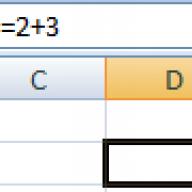
You must enter the formula with an equal sign. This is necessary so that Excel understands that it is the formula that is being entered into the cell, and not the data.
Select an arbitrary cell, for example A1. In the formula bar, enter =2+3 and press Enter. The result (5) will appear in the cell. And the formula itself will remain in the formula bar.
Experiment with different arithmetic operators: addition (+), subtraction (-), multiplication (*), division (/). To use them correctly, you need to clearly understand their priority.
The expressions inside the parentheses are executed first.
Multiplication and division have higher precedence than addition and subtraction.
Operators with the same precedence are executed from left to right.
My advice to you is USE BRACKETS. In this case, you will protect yourself from accidental errors in calculations, on the one hand, and on the other hand, brackets make it much easier to read and analyze formulas. If the number of closing and opening brackets in the formula does not match, Excel will display an error message and offer a suggestion for correcting it. Immediately after entering the closing bracket, Excel displays the last pair of brackets in bold (or in a different color), which is very convenient when there are a lot of brackets in the formula.
Now let's let's try to work using references to other cells in formulas.
Enter the number 10 in cell A1, and the number 15 in cell A2. In cell A3, enter the formula =A1+A2. The sum of cells A1 and A2 - 25 will appear in cell A3. Change the values of cells A1 and A2 (but not A3!). After changing the values in cells A1 and A2, the value of cell A3 is automatically recalculated (according to the formula).

In order not to make mistakes when entering cell addresses, you can use the mouse when entering links. In our case, we need to do the following:
Select cell A3 and enter the equal sign in the formula bar.
Click on cell A1 and enter a plus sign.
Click on cell A2 and press Enter.
The result will be the same.
Relative, absolute and mixed links


To better understand the link differences, let's experiment.
A1 - 20 B1 - 200
A2 - 30 B2 - 300
In cell A3, enter the formula =A1+A2 and press Enter.

Now place the cursor on the lower right corner of cell A3, press the right mouse button and drag to cell B3 and release the mouse button. A context menu will appear in which you need to select "Copy Cells".

After that, the formula value from cell A3 will be copied to cell B3. Activate cell B3 and see what formula you get - B1 + B2. Why did it happen? When we wrote the formula A1 + A2 in cell A3, Excel interpreted this entry as follows: "Take the values from the cell located in the current column two rows higher and add to the value of the cell located in the current column one row higher." Those. copying the formula from cell A3, for example, into cell C43, we get - C41 + C42. This is the beauty of relative links, the formula, as it were, adapts itself to our tasks.

Enter the following values in the cells:
A1 - 20 B1 - 200
A2 - 30 B2 - 300
Enter the number 5 in cell C1.
In cell A3, enter the following formula =A1+A2+$C$1. Copy the formula from A3 to B3 in the same way. See what happened. Relative links "adjusted" to the new values, but the absolute one remained unchanged.

Now try experimenting with mixed links yourself and see how they work. You can refer to other sheets in the same workbook just as you would to cells in the current sheet. You can even link to sheets in other books. In this case, the link will be called an external link.
For example, to write in cell A1 (Sheet 1) a link to cell A5 (Sheet 2), you need to do the following:
Select cell A1 and enter the equal sign;
Click on the label "Sheet 2";
Click on cell A5 and press the enter key;
after that, Sheet 1 will be activated again and the following formula will appear in cell A1 = Sheet2! A5.
Editing formulas is similar to editing text values in cells. Those. it is necessary to activate the cell with the formula by selection or double-clicking, and then edit it using, if necessary, the Del, Backspace keys. Committing changes is done with the Enter key.
Using text in formulas
You can perform mathematical operations on text values if the text values contain only the following characters:
Numbers from 0 to 9, + - e E /
You can also use five numeric formatting characters:
$ % () space
In this case, the text must be enclosed in double quotes.
Wrong: =$55+$33
Correct: ="$55"+$"33"
When performing calculations, Excel converts numeric text to numeric values, so the result of the above formula is 88.
The text operator & (ampersand) is used to concatenate text values. For example, if cell A1 contains the text value "Ivan", and cell A2 - "Petrov", then entering the following formula in cell A3 =A1&A2, we get "IvanPetrov".
To insert a space between the first and last name, write: =A1&" "&A2.
The ampersand can be used to combine cells with different data types. So, if cell A1 contains the number 10, and cell A2 contains the text "bags", then as a result of the formula =A1&A2, we get "10bags". Moreover, the result of such a union will be a text value.
Excel Functions - Introduction
Functions
AutoSum
Using headings in formulas
Functions
Functionexcel is a predefined formula that operates on one or more values and returns a result.
The most common Excel functions are shorthand for commonly used formulas.
For example function =SUM(A1:A4) similar to the entry =A1+A2+A3+A4.
And some functions perform very complex calculations.
Each function is made up of name And argument.
In the previous case SUM- This Name functions, and A1:A4-argument. The argument is enclosed in parentheses.
AutoSum
Because Since the sum function is used most often, the "Autosum" button has been placed on the "Standard" toolbar.
Enter arbitrary numbers in cells A1, A2, A3. Activate cell A4 and press the autosum button. The result is shown below.

Press the enter key. The formula for the sum of cells A1..A3 will be inserted into cell A4. The AutoSum button has a drop-down list from which you can select a different formula for the cell.
To select a function, use the "Insert function" button in the formula bar. When pressed, the following window appears.

If you don't know exactly what function you want to apply at the moment, you can search in the "Search for Function" dialog box.
If the formula is very cumbersome, then you can include spaces or line breaks in the text of the formula. This does not affect the calculation results in any way. To break a line, press Alt+Enter.
Using headings in formulas
You can use table headers instead of references to table cells in formulas. Build the following example.

By default, Microsoft Excel does not recognize headings in formulas. To use headings in formulas, choose Options on the Tools menu. On the Calculations tab, in the Book Options group, select the Allow range names check box.
In normal writing, the formula in cell B6 would look like this: \u003d SUM (B2: B4).
When using headings, the formula will look like this: \u003d SUM (Q 1).
You need to know the following:
If a formula contains the header of the column/row it is in, then Excel assumes that you want to use the range of cells below the table column header (or to the right of the row header);
If a formula contains a different column/row header than the one it is in, Excel assumes that you want to use the cell at the intersection of the column/row with that header and the row/column where the formula is located.
When using headings, you can specify any cell in the table using - range intersections. For example, to refer to cell C3 in our example, you can use the formula =Row2 Sq 2. Notice the space between the row and column headings.
Formulas containing headings can be copied and pasted, and Excel automatically adjusts them to the desired columns and rows. If an attempt is made to copy the formula to the wrong place, Excel will report this and display the value NAME? in the cell. When changing the names of the headings, similar changes occur in the formulas.
«Data entry in Excel || Excel || Excel Cell Names
Cell and range names inexcel
- Names in formulas
- Naming in the name field
- Rules for naming cells and ranges
Excel cells and ranges of cells can be named and then used in formulas. While formulas containing headings can only be used in the same worksheet as the table, range names can refer to table cells anywhere in any workbook.
Names in formulas
The name of a cell or range can be used in a formula. Let us have the formula A1 + A2 in cell A3. If you name cell A1 "Basic" and cell A2 - "Supplement", then the entry Base + Superstructure will return the same value as the previous formula.
Naming the name field
To assign a name to a cell (a range of cells), select the corresponding element, and then enter a name in the name field, while spaces cannot be used.
If the selected cell or range has been given a name, the name field displays that name, not the cell reference. If a name is defined for a range of cells, it will only appear in the name box when the entire range is selected.
If you want to navigate to a named cell or range, click the arrow next to the name field and select the name of the cell or range from the drop-down list.

More flexible options for naming cells and their ranges, as well as titles, are provided by the "Name" command from the "Insert" menu.
Cell and Range Naming Rules
The name must start with a letter, a backslash (\), or an underscore (_).
Only letters, numbers, backslashes, and underscores can be used in the name.
You cannot use names that can be interpreted as cell references (A1, C4).
Single letters can be used as names, except for the letters R,C.
Spaces must be replaced with underscores.
"Excel Functions|| Excel || Arrays Excel»
Arraysexcel
- Using arrays
- Two-dimensional arrays
- Rules for array formulas
Arrays in Excel are used to create formulas that return a set of results or operate on a set of values.
Using Arrays
Let's look at a few examples in order to better understand arrays.
Let's calculate, using arrays, the sum of the values in the rows for each column. To do this, do the following:
Enter numeric values in the range A1:D2.
Select the range A3:D3.
In the formula bar, enter =A1:D1+A2:D2.
Press the key combination Ctrl+Shift+Enter.

Cells A3:D3 form an array range, and the array formula is stored in each cell of this range. The array of arguments are references to the ranges A1:D1 and A2:D2
2D arrays
In the previous example, array formulas were placed in a horizontal one-dimensional array. You can create arrays that contain multiple rows and columns. Such arrays are called two-dimensional.

Rules for array formulas
Before entering an array formula, you must select the cell or range of cells that will contain the results. If the formula returns multiple values, you must select a range that is the same size and shape as the source data range.
Press Ctrl+Shift+Enter to commit the input of an array formula. This causes Excel to wrap the formula in curly braces in the formula bar. DO NOT MANUALLY ENTER CURLY BRACES!
In a range, you cannot edit, clear, or move individual cells, or insert or delete cells. All cells in the range of the array must be considered as a single unit and edited all of them at once.
To change or clear an array, select the entire array and activate the formula bar. After changing the formula, press the key combination Ctrl+Shift+Enter.
To move the contents of an array range, select the entire array and select the Cut command from the Edit menu. Then select the new range and choose Paste from the Edit menu.
You are not allowed to cut, clear, or edit part of an array, but you can assign different formats to individual cells in an array.
"Excel Cells and Ranges|| Excel || Formatting in Excel »
Assigning and removing formats inexcel
- Format assignment
- Delete format
- Formatting with toolbars
- Formatting individual characters
- Apply autoformat
Formatting in Excel is used to facilitate the perception of data, which plays an important role in productivity.
Format Purpose
Select the command "Format" - "Cells" (Ctrl + 1).
In the dialog box that appears (the window will be discussed in detail later), enter the desired formatting options.
Click the "OK" button
A formatted cell retains its format until a new format is applied to it or the old one is deleted. When you enter a value into a cell, the format already used in the cell is applied to it.
Deleting a format
Select a cell (range of cells).
Select the command "Edit" - "Clear" - "Formats".
To delete values in cells, select the "All" command from the "Clear" submenu.
Keep in mind that when you copy a cell, along with its contents, the format of the cell is also copied. Thus, you can save time by formatting the original cell before using the copy and paste commands.
Formatting with toolbars
The most frequently used formatting commands are placed on the "Formatting" toolbar. To apply a format using a toolbar button, select a cell or range of cells, and then click the button. To delete a format, press the button again.
To quickly copy formats from selected cells to other cells, you can use the Format Painter button on the Formatting toolbar.
Formatting individual characters
Formatting can be applied to individual characters of a text value in a cell in the same way as it can be applied to an entire cell. To do this, select the desired characters and then select the "Cells" command from the "Format" menu. Set the desired attributes and click OK. Press the Enter key to see the results of your work.
Applying AutoFormat
Excel automatic formats are predefined combinations of number format, font, alignment, borders, pattern, column width, and row height.
To use autoformat, follow these steps:
Enter the required data in the table.
Select the range of cells you want to format.
From the Format menu, select AutoFormat. This will open a dialog box.

In the AutoFormat dialog box, click the Options button to display the Edit area.
Select the appropriate auto-format and click OK.
Select a cell outside the table to deselect the current block and you will see the formatting results.

"Excel Arrays|| Excel || Formatting Numbers in Excel »
Format numbers and text in Excel
-General format
-Number formats
-Money formats
-Financial formats
-Percentage formats
- Fractional formats
- Exponential formats
-Text format
-Additional formats
-Creation of new formats
The "Format Cells" dialog box (Ctrl+1) allows you to control the display of numerical values and change the text output.
Before opening the dialog box, select the cell containing the number you want to format. In this case, the result will always be visible in the "Sample" field. Keep in mind the difference between stored and displayed values. Stored numeric or text values in cells are not affected by formats.

General format
Any text or numeric value entered is displayed in the General format by default. In this case, it is displayed exactly as it was entered into the cell, with the exception of three cases:
Long numeric values are displayed in exponential notation or rounded off.
The format does not display trailing zeros (456.00 = 456).
A decimal entered without a number to the left of the decimal point is output with a zero (,23 = 0.23).
Numeric formats
This format allows you to output numeric values as integers or fixed-point numbers, and highlight negative numbers with color.
Money formats
These formats are similar to number formats, except that instead of a thousands separator, they allow you to control the output of the currency symbol, which you can select from the Symbol list.
Financial formats
The financial format basically corresponds to the currency formats - you can display a number with or without a currency unit with a given number of decimal places. The main difference is that the financial format displays the currency left-aligned, while the number itself is right-aligned in the cell. As a result, both the currency and the numbers are vertically aligned in the column.
Percentage formats
This format displays numbers as percentages. The decimal point in the formatted number is shifted two places to the right, and the percent sign is displayed at the end of the number.
Fractional formats
This format outputs fractional values as fractions rather than decimals. These formats are especially useful when watering stock prices or measurements.
Exponential formats
Scientific formats display numbers in exponential notation. This format is very useful for displaying and displaying very small or very large numbers.
Text format
Applying a text format to a cell means that the value in that cell should be treated as text, as evidenced by left-alignment of the cell.
It doesn't matter if the numeric value is formatted as text, because Excel is capable of recognizing numeric values. An error will occur if a cell that has a text format contains a formula. In this case, the formula is treated as plain text, so errors are possible.
Additional formats
Creation of new formats
To create a format based on an existing format, do the following:
Select the cells to be formatted.
Press the key combination Ctrl + 1 and on the "Number" tab of the dialog box that opens, select the "All formats" category.
In the Type list, select the format you want to change and edit the contents of the field. This will keep the original format unchanged and add the new format to the Type list.
"Formatting in Excel || Excel ||
Aligning the contents of Excel cells
- Align left, center and right
-Filling cells
-Word wrap and justify
-Vertical alignment and text orientation
-Auto-size characters
The Alignment tab of the Format Cells dialog box controls the arrangement of text and numbers in cells. This tab can also be used to create multi-line labels, repeat a series of characters in one or more cells, change text orientation.

Align left, center and right
When you select Align Left, Align Center, or Align Right, the contents of the selected cells are aligned to the left, center, or right of the cell, respectively.

When left-aligned, you can change the amount of indentation, which defaults to zero. Increasing the indent by one unit moves the value in the cell one character width to the right, which is approximately the width of a capital X in the Normal style.
Filling cells
The Filled format repeats the value entered in the cell to fill the full width of the column. For example, in the worksheet shown in the figure above, cell A7 repeats the word "Fill". Although the range of cells A7-A8 appears to contain many words "Fill", the formula bar suggests that there is actually only one word. Like all other formats, the Filled format only affects the appearance, not the stored content of the cell. Excel repeats characters across the entire range with no gaps between cells.
It may seem that repeating characters are as easy to type with the keyboard as they are with padding. However, the Filled format provides two important advantages. First, if you adjust the column width, Excel increments or decrements the number of characters in the cell as appropriate. Secondly, you can repeat a character or characters in several neighboring cells at once.
Since this format affects numeric values in the same way as text, the number may look completely different from what it should be. For example, if you apply this format to a cell that is 10 characters wide and contains the number 8, that cell will display 8888888888.
Word wrap and justify
If you enter a label that is too long for the active cell, Excel expands the label beyond the cell, provided that adjacent cells are empty. If you then on the "Alignment" tab, check the "Wrap by words" box, Excel will display this inscription completely within one cell. To do this, the program will increase the height of the line in which the cell is located, and then place the text on additional lines inside the cell.

When using the Justify horizontal alignment format, the text in the active cell is word-wrapped on additional lines within the cell and aligned to the left and right edges with automatic line height adjustment.
If you create a multi-line text box and subsequently clear the Wrap By Words check box or use a different horizontal alignment format, Excel restores the original line height.
The "By Height" vertical alignment format does essentially the same thing as its "By Width" counterpart, except that it aligns the cell's value with respect to its top and bottom edges rather than its sides.
Vertical alignment and text orientation
Excel provides four vertical text alignment formats: top, center, bottom, height.

The Orientation area lets you position cell content vertically from top to bottom or obliquely up to 90 degrees clockwise or counterclockwise. Excel automatically adjusts the row height for vertical orientation unless you manually set the row height yourself earlier or later.
Auto-size characters
The "AutoFit Width" checkbox reduces the size of the characters in the selected cell so that its contents fit entirely in the column. This can be useful when working with a worksheet in which setting the column width to long has an undesirable effect on the rest of the data, or in that case. When using vertical or italic text, word wrap is not an acceptable solution. In the figure below, cells A1 and A2 have the same text entered, but Cell A2 has the AutoFit check box selected. When changing the column width, the size of the characters in cell A2 will decrease or increase accordingly. However, this preserves the font size assigned to the cell, and if you increase the column width beyond a certain value, the character size will not be adjusted.

It should be said that although this format is a good way to solve some problems, it must be borne in mind that the size of the characters can be arbitrarily small. If the column is narrow and the value is long enough, then after applying this format, the contents of the cell may become unreadable.
"Custom Format || Excel || Font in Excel»
Using cell borders and shadingexcel
-Using borders
-Apply colors and patterns
-Use fill
Using Borders
Cell borders and shading can be a good way to decorate different areas of a worksheet or draw attention to important cells.

To select a line type, click on any of the thirteen types of border line, including four solid lines of different thicknesses, a double line, and eight types of dashed lines.
By default, the color of the border line is black when the Color field is set to Auto on the View tab of the Options dialog box. To select a color other than black, click the arrow to the right of the Color field. The current 56-color palette will open, allowing you to use one of the available colors or define a new one. Note that you must use the "Color" list on the "Border" tab to select the border color. If you try to do this using the formatting toolbar, you will change the color of the text in the cell, not the color of the border.
After choosing the type and color of the line, you need to specify the position of the border. When you click the "Outer" button in the "All" area, the border is placed around the perimeter of the current selection, whether it is a single cell or a block of cells. To remove all borders from the selection, click the None button. The viewport allows you to control the placement of the borders. When you first open the dialog box for a single selected cell, this area contains only small handles that indicate the corners of the cell. To place a border, click on the viewport where the border should be, or click the appropriate button next to the region. If several cells are selected in the worksheet, then the "Internal" button becomes available on the "Border" tab, with which you can add borders between the selected cells. In addition, additional markers appear in the viewport on the sides of the selection, indicating where the inner boundaries will go.
To remove a placed border, simply click on it in the viewport. If you want to change the format of the border, select a different line type or color and click that border in the preview area. If you want to start placing borders again, click the No button in the All area.
You can apply several types of borders to selected cells at the same time.


You can apply border combinations using the Borders button on the Formatting toolbar. When you click on the small arrow next to this button, Excel will display a border palette where you can choose the type of border.

The palette consists of 12 border options, including combinations of different types, such as a single top border and a double bottom border. The first option in the palette removes all border formats in the selected cell or range. Other options show a thumbnail of the location of a border or a combination of borders.
As a practice, try to make a small example below. To break a line, you must press the Enter key while pressing Alt.

Applying color and patterns
The View tab of the Format Cells dialog box is used to apply color and patterns to selected cells. This tab contains the current palette and a drop-down pattern palette.

The Color palette on the View tab lets you set the background for selected cells. If you select a color in the Color palette without selecting a pattern, the specified background color will appear in the selected cells. If you select a color in the Color palette and then a pattern in the Pattern drop-down palette, that pattern is superimposed on the background color. The colors in the Pattern drop-down palette control the color of the pattern itself.
Using a fill
The various cell shading options provided by the View tab can be used to visually design your worksheet. For example, shading can be used to highlight summary data, or to draw attention to data entry cells on a worksheet. To make it easier to view numerical data by row, you can use the so-called "stripe fill" when rows of different colors alternate.

Choose a cell background color that makes it easy to read text and numbers displayed in the default black font.
Excel allows you to add a background image to your worksheet. To do this, select the command "Sheet" - "Substrate" from the "Format" menu. A dialog box will appear allowing you to open a graphic file stored on disk. This graphic is then used as the background of the current worksheet, similar to watermarks on a piece of paper. The graphic image is repeated if necessary until the entire worksheet is filled. You can disable the display of grid lines in the sheet, to do this, in the "Tools" menu, select the "Options" command and on the "View" tab and uncheck the "Grid" box. Cells that are assigned a color or pattern display only the color or pattern, not a graphical background image.

"Excel Font|| Excel || Merging Cells »
Conditional Formatting and Merging Cells
- Conditional formatting
- Merge cells
- Conditional formatting
Conditional formatting allows you to apply formats to specific cells that remain dormant until the values in those cells reach some control value.
Select the cells to be formatted, then from the "Format" menu, select the "Conditional Formatting" command, you will see the dialog box shown below.

The first combo box in the Conditional Formatting dialog box lets you choose whether the condition should be applied to the value or the formula itself. Typically, the Value option is selected, in which the format applied depends on the values of the selected cells. The Formula option is useful when you want to specify a condition that uses data from unselected cells, or you need to create a complex condition that includes multiple criteria. In this case, in the second combo box, enter a logical formula that takes the value TRUE or FALSE. The second combo box is used to select the comparison operator used to set the formatting condition. The third field is used to set the value to be compared. If the operator "Between" or "Outside" is selected, then an additional fourth field appears in the dialog box. In this case, the lower and upper values must be specified in the third and fourth fields.
After setting the condition, click the "Format" button. The Format Cells dialog box opens, allowing you to select the font, borders, and other format attributes that should be applied when the specified condition is met.
In the example below, the following format is set: font color - red, font - bold. Condition: if the value in the cell is greater than "100".

Sometimes it's hard to tell where conditional formatting has been applied. To select all cells with conditional formatting in the current worksheet, choose the Go command from the Edit menu, click the Select button, then select the Conditional Format radio button.

To remove a formatting condition, select a cell or range, and then choose Conditional Formatting from the Format menu. Specify the conditions you want to remove and click OK.

Merging cells
The grid is a very important design element in spreadsheet design. Sometimes, to achieve the desired effect, it is necessary to format the mesh in a special way. Excel allows you to merge cells, which gives the grid new features that you can use to create clearer forms and reports.
When cells are merged, one cell is formed, the dimensions of which coincide with the dimensions of the original selection. The merged cell gets the address of the top left cell of the original range. The remaining original cells practically cease to exist. If a formula contains a reference to such a cell, it is treated as empty, and depending on the type of formula, the reference may return a null or erroneous value.
To merge cells, do the following:
Select source cells;
In the "Format" menu, select the "Cells" command;
On the "Alignment" tab of the "Format Cells" dialog box, check the "Merge Cells" box;
Press "OK".


If this command has to be used quite often, then it is much more convenient to "pull" it to the toolbar. To do this, select the "Tools" - "Settings ..." menu, in the window that appears, go to the "Commands" tab and select the "Formatting" category in the right window. In the left "Commands" window, using the scroll bar, find "Cell Merge" and drag this icon (using the left mouse button) to the "Formatting" toolbar.

Merging cells has a number of consequences, most notably breaking the grid, one of the main attributes of spreadsheets. In this case, some nuances should be taken into account:
If only one cell in the selected range is non-empty, then when merged, its contents are relocated in the merged cell. So, for example, when merging cells in the range A1:B5, where cell A2 is non-empty, this cell will be transferred to the merged cell A1;
If multiple cells in the selected range contain values or formulas, then only the contents of the top left cell are retained when merged and are relocated in the merged cell. The contents of the remaining cells are deleted. If you need to save data in these cells, then before merging, you should add them to the upper left cell or move them to another place outside the selection;
If the merging range contains a formula that is relocated in the merged cell, the relative references in the merged cell are automatically adjusted;
Merged Excel cells can be copied, cut and pasted, deleted, and dragged just like normal cells. After copying or moving a merged cell, it occupies the same number of cells in the new location. In place of the cut or deleted merged cell, the standard cell structure is restored;
When cells are merged, all borders are removed, except for the outer border of the entire selection, as well as the border that is applied to any edge of the entire selection.
"Borders and shading || Excel || Editing"
Cutting and pasting cells inexcel
Cut and paste
Cut and paste rules
Insert cut cells
Cut and paste
The Cut and Paste commands on the Edit menu can be used to move values and formats from one place to another. Unlike the Delete and Clear commands, which delete cells or their contents, the Cut command places a movable dashed border around the selected cells and places a copy of the selection on the clipboard, which saves the data so that it can be pasted into another place.
After selecting the range into which to move the cut cells, the Paste command places them in a new location, clears the contents of the cells inside the moving frame, and removes the moving frame.
When you use the Cut and Paste commands to move a range of cells, Excel cleans up the content and formats in the cut range and moves them to the paste range.
When you do this, Excel adjusts any formulas outside the clipping region that refer to those cells.


Cut and paste rules
The selected cutout area must be a single rectangular block of cells;
When using the "Cut" command, the paste is performed only once. To paste the selected data into several places, use the "Copy"-"Clear" command combination;
It is not necessary to select the entire paste range before using the Paste command. When you select one cell as the paste range, Excel expands the paste area to match the size and shape of the area being cut. The selected cell is considered to be the top left corner of the insertion area. If the entire paste area is selected, then you need to make sure that the selected range has the same size as the cut area;
When you use the Paste command, Excel replaces the content and formats in all existing cells in the pasting range. If you don't want to lose the contents of existing cells, make sure that there are enough empty cells in the worksheet to accommodate the entire cutout area, below and to the right of the selected cell, which will end up in the upper left corner of the screen area.
Insert cut cells
When you use the Paste command, Excel inserts the cut cells into the selected area of the worksheet. If the selected area already contains data, then they are replaced by the inserted values.
In some cases, you can paste clipboard content between cells instead of placing it in existing cells. To do this, use the "Cut Cells" command of the "Insert" menu instead of the "Paste" command of the "Edit" menu.
The "Cut Cells" command replaces the "Cells" command and appears only after deleting data to the clipboard.
For example, in the example below, cells A5:A7 were originally cut (the "Cut" command of the "Edit" menu); then cell A1 was made active; then executed the "Cut Cells" command from the "Insert" menu.


"Filling rows || Excel || Excel Functions»
Functions. Function Syntaxexcel
Function Syntax
Using Arguments
Argument types
In lesson number 4, we already made the first acquaintance with Excel functions. Now it's time to take a closer look at this powerful spreadsheet toolkit.
Excel functions are special, pre-built formulas that allow you to easily and quickly perform complex calculations. They can be compared with special keys on calculators designed to calculate square roots, logarithms, and so on.
Excel has several hundred built-in functions that perform a wide range of different calculations. Some functions are the equivalent of long math formulas that you can do yourself. And some functions in the form of formulas cannot be implemented.
Function Syntax
Functions consist of two parts: the name of the function and one or more arguments. The name of a function, such as SUM, describes the operation that this function performs. The arguments specify the values or cells used by the function. In the formula below: SUM is the name of the function; B1:B5 - argument. This formula sums up the numbers in cells B1, B2, B3, B4, B5.
SUM(B1:B5)
An equal sign at the beginning of a formula means that the formula is entered, not text. If there is no equal sign, then Excel will treat the input as just text.
The function argument is enclosed in parentheses. An opening parenthesis marks the start of an argument and is placed immediately after the function name. If you enter a space or other character between the name and the opening bracket, the cell will display the erroneous value #NAME? Some functions take no arguments. Even in this case, the function must contain parentheses:
Using Arguments
When multiple arguments are used in a function, they are separated from one another by a semicolon. For example, the following formula indicates that you need to multiply the numbers in cells A1, A3, A6:
PRODUCT(A1, A3, A6)
You can use up to 30 arguments in a function, as long as the total length of the formula does not exceed 1024 characters. However, any argument can be a range containing an arbitrary number of worksheet cells. For example:
Argument types
In the previous examples, all of the arguments were cell or range references. But you can also use numeric, text, boolean, range names, arrays, and erroneous values as arguments. Some functions return values of these types, and they can later be used as arguments in other functions.
Numeric values
Function arguments can be numeric. For example, the SUM function in the following formula adds the numbers 24, 987, 49:
SUM(24;987;49)
Text values
Text values can be used as a function argument. For example:
TEXT(TDATE(); "D MMM YYYY")
In this formula, the second argument to the TEXT function is text and specifies a template for converting the decimal date value returned by the NOW(NOW) function to a character string. The text argument can be a character string enclosed in double quotes, or a cell reference that contains text.
Boolean values
Arguments to some functions can only take the boolean values TRUE or FALSE. The boolean expression returns TRUE or FALSE in the cell or formula that contains the expression. For example:
IF(A1=TRUE;"Increase","Decrease")&"prices"
You can specify the name of a range as an argument to the function. For example, if the cell range A1:A5 is named "Debit" (Insert-Name-Assign), then to calculate the sum of the numbers in cells A1 through A5, you can use the formula
SUM(Debit)
Using Different Types of Arguments
You can use different types of arguments in the same function. For example:
AVERAGE(Debit;C5;2*8)
"Insert Cells || Excel || Entering Excel Functions »
Entering Functions in a Worksheetexcel
You can enter functions in a worksheet directly from the keyboard or using the "Function" command of the "Insert" menu. When entering a function from the keyboard, it is better to use lowercase letters. When you finish entering a function, Excel will change the letters in the function name to uppercase if it was entered correctly. If the letters do not change, then the function name was entered incorrectly.
If you select a cell and select Function from the Insert menu, Excel displays the Function Wizard dialog box. You can achieve this a little faster by pressing the function icon key in the formula bar.


You can also open this window using the "Insert function" button on the standard toolbar.
In this window, first select a category from the "Category" list, and then select the desired function from the "Function" alphabetical list.
Excel will enter an equal sign, the name of the function, and a pair of parentheses. Excel will then open a second Function Wizard dialog box.

The second dialog box of the Function Wizard contains one field for each argument of the selected function. If the function has a variable number of arguments, this dialog box expands when additional arguments are given. The description of the argument whose field contains the insertion point is displayed at the bottom of the dialog box.
To the right of each argument field, its current value is displayed. This is very handy when you use links or names. The current value of the function is displayed at the bottom of the dialog box.
Click the "OK" button and the created function will appear in the formula bar.

"Syntax of functions || Excel || Math Functions»
Math functionsexcel
Here are the most commonly used Excel math functions (quick reference). Additional information about functions can be found in the Function Wizard dialog box, as well as in the Excel help system. In addition, many mathematical functions are included in the Analysis ToolPak.
SUM function (SUM)
EVEN and ODD functions
Functions FRAMEDOWN, FRAMEUP
INTEGER and SELECT functions
RAND and RANDBETWEEN functions
PRODUCT function
MOD function
ROOT function
COMBIN function
ISNUMBER function
LOG function
LN function
EXP function
PI function
RADIANS and DEGREES function
SIN function
COS function
TAN function
SUM function (SUM)
The SUM function adds up a set of numbers. This function has the following syntax:
SUM(numbers)
The number argument can have up to 30 elements, each of which can be a number, a formula, a range, or a cell reference that contains or returns a numeric value. The SUM function ignores arguments that refer to empty cells, text, or Boolean values. The arguments do not have to form contiguous ranges of cells. For example, to get the sum of the numbers in cells A2, B10, and cells C5 through K12, enter each link as a separate argument:
SUM(A2,B10,C5:K12)
ROUND, ROUNDDOWN, ROUNDUP functions
The ROUND function rounds the number given by its argument to the specified number of decimal places and has the following syntax:
ROUND(number, number_of_digits)
The number argument can be a number, a cell reference that contains a number, or a formula that returns a numeric value. The num_digits argument, which can be any positive or negative integer, determines how many digits to round. Specifying a negative number_digits argument rounds to the specified number of digits to the left of the decimal point, while setting the number_digits argument to 0 rounds to the nearest whole number. Excel numbers that are less than 5 are deficient (down), and numbers that are greater than or equal to 5 are in excess (up).
The ROUNDDOWN and ROUNDUP functions have the same syntax as the ROUND function. They round values down (under) or up (over).
EVEN and ODD functions
To perform rounding operations, you can use the EVEN (EVEN) and ODD (ODD) functions. The EVEN function rounds a number up to the nearest even integer. The ODD function rounds a number up to the nearest odd integer. Negative numbers are rounded down, not up. Functions have the following syntax:
EVEN(number)
ODD(number)
Functions FRAMEDOWN, FRAMEUP
The FLOOR and CEILING functions can also be used to perform rounding operations. The FIRMWARE function rounds a number down to the nearest multiple of a given factor, and the FIRMWARE function rounds a number up to the nearest multiple of a given factor. These functions have the following syntax:
FLOOR(number, multiplier)
CURUP(number, multiplier)
The number and multiplier values must be numeric and have the same sign. If they have different characters, an error will be thrown.
INTEGER and SELECT functions
The INT function rounds a number down to the nearest integer and has the following syntax:
INTEGER(number)
The number argument is the number for which to find the next smallest integer.
Consider the formula:
INTEGER(10,0001)
This formula will return the value 10, just like the following:
WHOLE(10,999)
The TRUNC function discards all digits to the right of the decimal point, regardless of the sign of the number. The optional argument number_digits specifies the position after which truncation is performed. The function has the following syntax:
SELECT(number,number_of_digits)
If the second argument is omitted, it is assumed to be zero. The following formula returns the value 25:
OBR(25,490)
The ROUND, INTEGER, and REFERENCE functions remove unnecessary decimal places, but they work differently. The ROUND function rounds up or down to the specified number of decimal places. The INT function rounds down to the nearest whole number, while the SET function discards decimal places without rounding. The main difference between the functions INTEGER and SELECT appears in the handling of negative values. If you use the value -10.900009 in the INT function, the result is -11, but if you use the same value in the SET function, the result is -10.
RAND and RANDBETWEEN functions
The RAND function generates random numbers evenly distributed between 0 and 1 and has the following syntax:
The RAND function is one of the EXCEL functions that take no arguments. As with all functions that take no arguments, parentheses must be included after the function name.
The value of the RAND function changes each time the worksheet is recalculated. If calculations are set to update automatically, the value of the RAND function changes each time data is entered in this worksheet.
The RANDBETWEEN function, which is available when the Analysis ToolPak is installed, provides more options than RANDBETWEEN. For the RANDBETWEEN function, you can specify the interval of generated random integer values.
Function syntax:
RANDBETWEEN(start, end)
The start argument specifies the smallest number that any integer from 111 to 529 can return (including both of these values):
RANDOMBETWEEN(111,529)
PRODUCT function
The PRODUCT function multiplies all the numbers given by its arguments and has the following syntax:
PRODUCT(number1,number2...)
This function can have up to 30 arguments. Excel ignores any empty cells, text and boolean values.
MOD function
The MOD (MOD) function returns the remainder of a division and has the following syntax:
MOD(number, divisor)
The value of the MOD function is the remainder obtained when the number argument is divided by a divisor. For example, the following function will return the value 1, which is the remainder obtained when 19 is divided by 14:
OSTAT(19;14)
If the number is less than the divisor, then the value of the function is equal to the number argument. For example, the following function will return the number 25:
OSTAT(25;40)
If the number is exactly divisible by the divisor, the function returns 0. If the divisor is 0, the MOD function returns an erroneous value.
ROOT function
The SQRT (SQRT) function returns the positive square root of a number and has the following syntax:
ROOT(number)
The number argument must be a positive number. For example, the following function returns the value 4:
ROOT(16)
If the number is negative, SQRT returns an error value.
COMBIN function
The COMBIN function determines the number of possible combinations or groups for a given number of elements. This function has the following syntax:
COMBIN(number,number_chosen)
The number argument is the total number of elements, and num_chosen is the number of elements in each combination. For example, to determine the number of teams with 5 players that can be formed from 10 players, the formula is used:
COMBIN(10;5)
The result will be 252. That is, 252 teams can be formed.
ISNUMBER function
The ISNUMBER function determines whether a value is a number and has the following syntax:
ISNUMBER(value)
Let's say you want to know if the value in cell A1 is a number. The following formula returns TRUE if cell A1 contains a number or a formula that returns a number; otherwise it returns FALSE:
NUMBER(A1)
LOG function
The LOG function returns the logarithm of a positive number to the given base. Syntax:
LOG(number; base)
If the base argument is not specified, then Excel assumes it is 10.
LN function
The LN function returns the natural logarithm of the positive number given as an argument. This function has the following syntax:
EXP function
The EXP function calculates the value of a constant raised to a given power. This function has the following syntax:
The EXP function is the inverse of LN. For example, let's say cell A2 contains the formula:
Then the following formula returns the value 10:
PI function
The PI function (PI) returns the value of the constant pi to 14 decimal places. Syntax:
RADIANS and DEGREES function
Trigonometric functions use angles expressed in radians, not degrees. The measurement of angles in radians is based on the constant pi and 180 degrees equals pi radians. Excel provides two functions, RADIANS and DEGREES, to help you work with trigonometric functions.
You can convert radians to degrees using the DEGREES function. Syntax:
DEGREES(angle)
Here - angle is a number representing an angle measured in radians. To convert degrees to radians, use the RADIANS function, which has the following syntax:
RADIANS(angle)
Here - angle is a number representing an angle measured in degrees. For example, the following formula returns the value 180:
DEGREES(3.14159)
At the same time, the following formula returns the value 3.14159:
RADIANS(180)
SIN function
The SIN function returns the sine of an angle and has the following syntax:
SIN(number)
COS function
The COS function returns the cosine of an angle and has the following syntax:
COS(number)
Here the number is the angle in radians.
TAN function
The TAN function returns the tangent of an angle and has the following syntax:
TAN(number)
Here the number is the angle in radians.
«Introduction of functions || Excel || Text Functions»
Text functionsexcel
Here are the most commonly used Excel text functions (quick reference). Additional information about functions can be found in the Function Wizard dialog box, as well as in the Excel help system.
TEXT function
RUBLE function
DLSTR function
CHAR and CODE CHAR function
TRIM and CLEAN functions
EXACT function
ETEXT and ENETEXT functions
Text functions convert numeric text values to numbers and numeric values to character strings (text strings), and also allow you to perform various operations on character strings.
TEXT function
The TEXT function converts a number into a text string with the given format. Syntax:
TEXT(value, format)
The value argument can be any number, formula, or cell reference. The format argument determines how the returned string is displayed. You can use any of the formatting characters except for the asterisk to specify the format you want. The use of the General format is not allowed. For example, the following formula returns the text string 25.25:
TEXT(101/4,"0.00")
RUBLE function
The RUBLE (DOLLAR) function converts a number to a string. However, RUBLE returns a currency string with the specified number of decimal places. Syntax:
RUBLE(number, number_of_digits)
In this case, Excel rounds the number if necessary. If the num_chars argument is omitted, Excel uses two decimal places, and if the value of this argument is negative, then the return value is rounded to the left of the decimal point.
DLSTR function
The LEN (LEN) function returns the number of characters in a text string and has the following syntax:
DLSTR(text)
The text argument must be a character string enclosed in double quotes or a cell reference. For example, the following formula returns the value 6:
DLSTR("head")
The DLSTR function returns the length of the displayed text or value, not the stored value of the cell. It also ignores leading zeros.
CHAR and CODE CHAR function
Any computer uses numeric codes to represent characters. The most common character encoding system is ASCII. In this system, numbers, letters, and other symbols are represented by numbers from 0 to 127 (255). The CHAR and CODE functions deal with ASCII codes. The CHAR function returns the character that corresponds to the specified ASCII numeric code, and the CODE function returns the ASCII code for the first character of its argument. Function syntax:
CHAR(number)
CODE(text)
If you enter a character as a text argument, be sure to enclose it in double quotes, otherwise Excel will return an erroneous value.
TRIM and CLEAN functions
Often, leading and trailing spaces prevent values from being sorted correctly in a worksheet or database. If you use text functions to work with worksheet texts, extra spaces can prevent formulas from working correctly. The TRIM function removes leading and trailing spaces from a string, leaving only one space between words. Syntax:
TRIM(text)
The CLEAN function is similar to the TRIM function, except that it removes all non-printable characters. The PRINT function is especially useful when importing data from other programs because some imported values may contain non-printable characters. These characters may appear on worksheets as small squares or vertical lines. The CLEAN function allows you to remove non-printable characters from such data. Syntax:
PRINT(text)
EXACT function
The EXACT function compares two lines of text for complete identity, case-sensitive. The formatting difference is ignored. Syntax:
EXACT(text1, text2)
If the arguments text1 and text2 are case-sensitive, the function returns TRUE; otherwise, FALSE. The text1 and text2 arguments must be character strings enclosed in double quotes, or cell references that contain text.
UPPER, LOWER, and PROPER functions
There are three functions in Excel that allow you to change the case of letters in text strings: UPPER, LOWER, and PROPER. The UPPER function converts all letters in a text string to uppercase, and LOWER to lowercase. The PROPER function capitalizes the first letter in each word and all letters immediately following non-letter characters; all other letters are converted to lowercase. These functions have the following syntax:
UPPER(text)
LOWER(text)
PROPER(text)
When working with already existing data, a situation often arises when you need to modify the original values themselves, to which text functions are applied. You can enter a function in the same cells where these values are, since the entered formulas will replace them. But you can create temporary formulas with a text function in free cells on the same line and copy the result to the clipboard. To replace the original values with the modified ones, select the original text cells, choose Paste Special from the Edit menu, select the Values radio button, and then click OK. After that, you can delete temporary formulas.
ETEXT and ENETEXT functions
The ISTEXT and ISNOTEXT functions check whether a value is a text value. Syntax:
ISTEXT(value)
ENETEXT(value)
Suppose you want to determine if the value in cell A1 is text. If cell A1 contains text or a formula that returns text, you can use the formula:
ETEXT(A1)
In this case, Excel returns the logical value TRUE. Similarly, if you use the formula:
ENETEXT(A1)
Excel returns the boolean value FALSE.
"Math Functions || Excel || String Functions»
Functionsexcelto work with row elements
FIND and SEARCH functions
RIGHT and LEFT functions
MID function
REPLACE and SUBSTITUTE functions
REPEAT function
CONCATENATE function
The following functions find and return parts of text strings or compose large strings from small ones: FIND (FIND), SEARCH (SEARCH), RIGHT (RIGHT), LEFT (LEFT), MID (MID), SUBSTITUTE (SUBSTITUTE), REPEAT (REPT), REPLACE (REPLACE), CONCATENATE (CONCATENATE).
FIND and SEARCH functions
The FIND and SEARCH functions are used to determine the position of one text string within another. Both functions return the character number from which the first occurrence of the searched string begins. The two functions work the same except that the FIND function is case-sensitive, while the SEARCH function accepts wildcard characters. Functions have the following syntax:
FIND(search_text, search_text, start_position)
SEARCH(search_text, search_text, start_position)
The search_text argument specifies the text string to be found, and the search_text argument specifies the text to search. Any of these arguments can be a character string enclosed in double quotes or a cell reference. The optional start_position argument specifies the position in the text being viewed at which to start the search. The start_position argument should be used when lookup_text contains multiple occurrences of the search text. If this argument is omitted, Excel returns the position of the first occurrence.
These functions return an error value when search_text is not contained in the search text, or start_position is less than or equal to zero, start_position is greater than the number of characters in the search text, or start_position is greater than the position of the last occurrence of the search text.
For example, to determine the position of the letter "g" in the string "Garage gate", you need to use the formula:
FIND("W", "Garage Door")
This formula returns 5.
If you don't know the exact sequence of characters you're looking for, you can use the SEARCH function and include the wildcard characters: question mark (?) and asterisk (*) in the search_text string. The question mark matches a single randomly typed character, and the asterisk matches any sequence of characters in the specified position. For example, to find the position of the names Anatoly, Alexey, Akakiy in the text in cell A1, you need to use the formula:
SEARCH("A*d", A1)
RIGHT and LEFT functions
The RIGHT function returns the rightmost characters of the argument string, while the LEFT function returns the first (left) characters. Syntax:
RIGHT(text, number_of_characters)
LEFT(text, number_of_characters)
The num_chars argument specifies the number of characters to extract from the text argument. These functions respect spaces, and therefore, if the text argument contains spaces at the beginning or end of the line, the function arguments should use the TRIM function.
The number_of_chars argument must be greater than or equal to zero. If this argument is omitted, Excel treats it as 1. If the number_of_characters is greater than the number of characters in the text argument, then the entire argument is returned.
MID function
The MID function returns a specified number of characters from a string of text, starting at a specified position. This function has the following syntax:
MID(text, start_position, number_of_characters)
The text argument is the text string containing the characters to be extracted, start_position is the position of the first character to be extracted from the text (relative to the beginning of the string), and num_chars is the number of characters to extract.
REPLACE and SUBSTITUTE functions
These two functions replace characters in text. The REPLACE function replaces part of a text string with another text string and has the syntax:
REPLACE(old_text, start_position, number_of_characters, new_text)
The old_text argument is the text string to replace characters with. The next two arguments specify the characters to be replaced (relative to the beginning of the string). The new_text argument specifies the text string to insert.
For example, cell A2 contains the text "Vasya Ivanov". To put the same text in cell A3, replacing the name, you need to insert the following function into cell A3:
REPLACE(A2, 1, 5, "Petya")
In the SUBSTITUTE function, the starting position and the number of characters to be replaced are not specified, but the replacement text is explicitly specified. The SUBSTITUTE function has the following syntax:
SUBSTITUTE(text, old_text, new_text, entry_number)
The entry_number argument is optional. It instructs Excel to replace only the given occurrence of the string old_text.
For example, cell A1 contains the text "Zero is less than eight." We need to replace the word "zero" with "null".
SUBSTITUTE(A1, "o", "y", 1)
The number 1 in this formula indicates that only the first "o" in the row of cell A1 needs to be changed. If occurrence_num is omitted, Excel replaces all occurrences of old_text with new_text.
REPEAT function
The REPEAT function (REPT) allows you to fill a cell with a string of characters repeated a specified number of times. Syntax:
REPEAT(text, number_of_repetitions)
The text argument is a multiplied string of characters enclosed in quotation marks. The number_of_repeat argument specifies how many times the text should be repeated. If the number_of_repeats argument is 0, the REPEAT function leaves the cell blank, and if it is not an integer, this function discards the decimal places after the decimal point.
CONCATENATE function
The CONCATENATE function is the equivalent of the text operator & and is used to concatenate strings. Syntax:
CONCATENATE(text1, text2,...)
You can use up to 30 arguments in a function.
For example, cell A5 contains the text "first half", the following formula returns the text "Total for the first half":
CONCATENATE("Total for ";A5)
"Text Functions || Excel || Logic functions"
Logic functionsexcel
IF function
AND, OR, NOT functions
Nested IF Functions
TRUE and FALSE functions
IS BLANK function
Boolean expressions are used to write conditions that compare numbers, functions, formulas, textual or boolean values. Any logical expression must contain at least one comparison operator that defines the relationship between the elements of the logical expression. Below is a list of Excel comparison operators
> More
< Меньше
>= Greater than or equal
<= Меньше или равно
<>Not equal
The result of a logical expression is the logical value TRUE (1) or the logical value FALSE (0).
IF function
The IF (IF) function has the following syntax:
IF(logical_expression, value_if_true, value_if_false)
The following formula returns 10 if the value in cell A1 is greater than 3, and 20 otherwise:
IF(A1>3;10;20)
You can use other functions as arguments to the IF function. You can use text arguments in the IF function. For example:
IF(А1>=4;"passed the test";"failed to pass the test")
You can use text arguments in the IF function so that if the condition is not met, it returns an empty string instead of 0.
For example:
IF(SUM(A1:A3)=30,A10,"")
The boolean_expression argument of the IF function can contain a text value. For example:
IF(A1="Dynamo";10;290)
This formula returns 10 if cell A1 contains the string "Dynamo", and 290 if it contains any other value. The match between the compared text values must be exact, but not case sensitive. AND, OR, NOT functions
Functions AND (AND), OR (OR), NOT (NOT) - allow you to create complex logical expressions. These functions work in conjunction with simple comparison operators. The AND and OR functions can have up to 30 Boolean arguments and have the syntax:
AND(boolean1, boolean2...)
OR(boolean1, boolean2...)
The NOT function has only one argument and the following syntax:
NOT(boolean_value)
The arguments of the AND, OR, NOT functions can be boolean expressions, arrays, or cell references containing boolean values.
Let's take an example. Let Excel return the text "Pass" if the student has a GPA greater than 4 (cell A2) and absenteeism is less than 3 (cell A3). The formula will look like:
IF(AND(A2>4,A3<3);"Прошел";"Не прошел")
Despite the fact that the OR function has the same arguments as the AND, the results are completely different. So, if in the previous formula we replace the AND function with OR, then the student will pass if at least one of the conditions is met (average score is more than 4 or absenteeism is less than 3). Thus, the OR function returns the logical value TRUE if at least one of the logical expressions is true, and the AND function returns the logical value TRUE only if all the logical expressions are true.
The function does NOT change the value of its argument to the opposite boolean value and is usually used in conjunction with other functions. This function returns Boolean TRUE if the argument is FALSE and Boolean FALSE if the argument is TRUE.
Nested IF Functions
Sometimes it can be very difficult to solve a logical problem only with the help of comparison operators and AND, OR, NOT functions. In these cases, nested IF functions can be used. For example, the following formula uses three IF functions:
IF(A1=100, "Always", IF(AND(A1>=80, A1<100);"Обычно";ЕСЛИ(И(А1>=60;A1<80);"Иногда";"Никогда")))
If the value in cell A1 is an integer, the formula reads as follows: "If the value in cell A1 is 100, return the string 'Always'. Otherwise, if the value in cell A1 is between 80 and 100, return 'Normal'. B otherwise, if the value in cell A1 is between 60 and 80, return the string “Sometimes.” And, if none of these conditions are met, return the string “Never.” In total, up to 7 levels of nesting of IF functions are allowed.
TRUE and FALSE functions
The TRUE and FALSE functions provide an alternative way to write the logical values TRUE and FALSE. These functions take no arguments and look like this:
For example, cell A1 contains a boolean expression. Then the following function will return "Pass" if the expression in cell A1 is TRUE:
IF(A1=TRUE();"Go";"Stop")
Otherwise, the formula will return "Stop".
IS BLANK function
If you want to determine if a cell is empty, you can use the ISBLANK function, which has the following syntax:
NULL(value)
"String Functions || Excel || Excel 2007"
This program is used by a large number of people. Andrey Sukhov decided to record a series of educational video lessons "Microsoft Excel for Beginners" for novice users and we invite you to familiarize yourself with the basics of this program.
Lesson 1
In the first lesson, Andrey will talk about the interface of the Excel program and its main elements. You will also understand the workspace of the program, with columns, rows and cells. So here's the first video:
Lesson 2: How to Enter Data in an Excel Spreadsheet
In the second video tutorial on the basics of Microsoft Excel, we will learn how to enter data into a spreadsheet, and also get acquainted with the auto-fill operation. I think that the most effective learning is the one built on practical examples. So we will begin to create a spreadsheet that will help us maintain a family budget. Based on this example, we will consider the tools of the Microsoft Excel program. So here's the second video:
Lesson 3. How to format spreadsheet cells in Excel
In the third video tutorial on the basics of Microsoft Excel, we will learn how to align the contents of the cells of our spreadsheet, as well as change the width of the columns and the height of the rows of the table. Next, we will get acquainted with the Microsoft Excel tools that allow you to merge table cells, as well as change the direction of text in cells if necessary. So here's the third video:
Lesson 4. How to format text in Excel
In the fourth video tutorial on the basics of Microsoft Excel, we will get acquainted with the text formatting operations. For different elements of our table, we will apply different fonts, different font sizes and text styles. We will also change the text color and set a colored background for some cells. At the end of the lesson, we will get an almost ready-made family budget form. So, the fourth video:
Lesson 5
In the fifth video tutorial on the basics of Microsoft Excel, we will finalize the family budget form that we started working on in previous lessons. In this lesson, we will talk about cell borders. We will set different borders for different columns and rows of our table. By the end of the lesson, we will have a family budget form completely ready for data entry. So, the fifth video:
Lesson 6
In the sixth video tutorial on the basics of Microsoft Excel, we will fill in our family budget form with data. Microsoft Excel allows you to simplify the process of data entry to the maximum, and we will get acquainted with these features. Next, I will talk about data formats in cells and how they can be changed. By the end of the lesson, we will receive a family budget form filled in with initial data. So, the sixth video:
Lesson 7
In the seventh video tutorial on the basics of Microsoft Excel, we will talk about the most interesting thing - about formulas and calculations. Microsoft Excel has a very powerful toolkit for performing various calculations. We will learn how to perform basic calculations using spreadsheets, then we will get acquainted with the function wizard, which greatly simplifies the process of creating formulas for performing calculations. So, the seventh video:
Lesson 8
In the eighth video tutorial on the basics of Microsoft Excel, we will completely finish working on the family budget template. We will compose all the necessary formulas and carry out the final formatting of rows and columns. The family budget form will be ready and if you keep your family budget, you will be able to adjust it to fit your expenses and income. So, the eighth video:
Lesson 9
In the final ninth lesson on the basics of Microsoft Excel, we will learn how to create charts and graphs. Microsoft Excel has a very impressive toolkit for visualizing the results of calculations. In the form of graphs, charts and histograms, you can present any data, both simply entered into a spreadsheet, and data obtained as a result of calculations. So, the final ninth video:
Most users of Windows-based computer systems with the Microsoft Office package installed will certainly come across the MS Excel application. For novice users, the program causes some difficulties in mastering, however, working in Excel with formulas and tables is not so difficult as it might seem at first glance, if you know the basic principles underlying the application.
What is Excel?
At its core, Excel is a full-fledged mathematical machine for performing many arithmetic, algebraic, trigonometric and other more complex operations, operating with several basic data types that are not always related specifically to mathematics.
Working with Excel spreadsheets means using more features with the combination of calculations, plain text, and multimedia. But in its original form, the program was created precisely as a powerful mathematical editor. Some, however, at first take the application for some kind of calculator with advanced features. Deepest delusion!
Work in Excel with tables for beginners: the first acquaintance with the interface
First of all, after opening the program, the user sees the main window, which contains the main controls and tools for work. In later versions, when the application starts, a window appears in which it is proposed to create a new file, by default called "Book 1" or select a template for further actions.
Working with Excel tables for beginners at the first stage of acquaintance with the program should come down to creating an empty table. For now, let's look at the main elements.

The main field is occupied by the table itself, which is divided into cells. Each is numbered, thanks to two-dimensional coordinates - the row number and the letter designation of the column (for example, we take Excel 2016). Such numbering is necessary so that in the dependency formula it is possible to clearly identify exactly the cell with data, the operation on which will be performed.
Above, as in other office applications, is the main menu bar, and a little lower is the toolkit. Under it there is a special line in which formulas are entered, and a little to the left you can see a window with the coordinates of the currently active cell (on which the rectangle is located). At the bottom there is a sheet panel and a horizontal slider, and below it there are buttons for switching the view and scaling. On the right is a vertical bar for moving up / down the sheet.
Basic data entry types and simple operations
At first, it is assumed that work in Excel with tables by a novice user will be mastered by operations familiar to him, for example, in the same Word text editor.
As usual, in the table, you can copy, cut or paste data, enter text or numeric data.

But the input is somewhat different from that produced in text editors. The fact is that the program is initially configured to automatically recognize what the user writes in the active cell. For example, if you enter the string 1/2/2016, the data will be recognized as a date, and the date will appear in the cell instead of the entered numbers in a simplified form - 02/01/2016. Changing the display format can be quite simple (we will dwell on this a little later).

The same is true with numbers. You can enter any numeric data, even with an arbitrary number of decimal places, and they will be displayed in the form in which everyone is used to seeing them. But, if an integer is entered, it will be presented without the mantissa (the decimal places as zeros). You can also change this.
But at the end of data entry, many novice users try to move to the next cell using the keyboard arrows for this (similar to how you can do it in Word tables). And it doesn't work. Why? Yes, only because working with Excel tables differs from the Word text editor quite noticeably. The transition can be done by pressing the Enter key or setting the active rectangle to another cell using the left mouse click. If, after writing something in the active cell, press the Esc key, the input will be canceled.
Sheet Actions
Working with sheets at first should not cause difficulties. On the panel below there is a special button for adding sheets, after clicking on which a new table will appear with automatic transition to it and setting a name (“Sheet 1”, “Sheet 2”, etc.).

By double-clicking, you can activate the renaming of any of them. You can also use the right-click menu to bring up an additional menu that has a few basic commands.
Cell Formats
Now the most important thing is that the cell format is one of the basic concepts, which determines the data type that will be used to recognize its contents. You can call format editing through the right-click menu, where the corresponding line is selected, or by pressing the F2 key.

The window on the left shows all available formats, and on the right shows the data display options. Looking at the date example shown above, the format is set to "Date" and the desired appearance is set to the right (for example, February 1, 2016).

Several formats can be used to perform mathematical operations, but in the simplest case, we will choose a numeric one. On the right there are several types of input, a pointer to the number of decimal places in the mantissa and a field for setting the separator of groups of digits. Using other number formats (exponential, fractional, monetary, etc.), you can also set the desired parameters.
By default, automatic data recognition is set to the general format. But when you enter text or several letters, the program can spontaneously convert it into something else. Therefore, to enter text for the active cell, you need to set the appropriate parameter.
Working in Excel with formulas (tables): an example
Finally, a few words about formulas. And to begin with, consider the example of the sum of two numbers located in cells A1 and A2. The application has an automatic summation button with some additional functions (calculating the arithmetic average, maximum, minimum, etc.). It is enough to set the active cell located in the same column below, and when you select the amount, it will be calculated automatically. The same works for horizontal values, but the active cell for the amount must be set to the right.

But you can also enter the formula manually (working with Excel tables also implies such a possibility when automatic action is not provided). For the same amount, put an equal sign in the formula bar and write the operation in the form A1 + A2 or SUM (A1; A2), and if you want to specify a range of cells, use this form after the equal sign: (A1: A20), after which it will be the sum of all numbers in cells from the first to the twentieth inclusive is calculated.
Construction of graphs and charts
Working with Excel tables is also interesting because it involves the use of a special automated tool for constructing dependency graphs and charts based on selected ranges.

To do this, there is a special button on the panel, after clicking on which you can select any parameters or the desired view. After that, the chart or graph will be displayed on the sheet as a picture.
Cross links, data import and export
The program can also establish data links located on different sheets, use files of a different format or objects located on servers on the Internet, and many other add-ons.

In addition, Excel files can be exported to other formats (for example, PDF), data can be copied from them, etc. But the program itself can also open files created in other applications (text formats, databases, web pages, XML- documents, etc.).
As you can see, the possibilities of the editor are almost unlimited. And, of course, there is simply not enough time to describe them all. Only the basics are given here, but the interested user will have to read the help information in order to master the program at the highest level.