In the second part of the Excel 2010 Beginner series, you'll learn how to link table cells with math formulas, add rows and columns to an existing table, learn about the AutoComplete feature, and more.
Introduction
In the first part of the "Excel 2010 for Beginners" series, we got acquainted with the very basics of Excel, having learned how to create ordinary tables in it. Strictly speaking, this is a simple matter and of course the possibilities of this program are much wider.
The main advantage of spreadsheets is that individual data cells can be linked together by mathematical formulas. That is, when the value of one of the interconnected cells changes, the data of the others will be recalculated automatically.
In this part, we will see how useful such opportunities can be using the example of the budget expenditure table we have already created, for which we will have to learn how to write simple formulas. We will also get acquainted with the autocomplete function of cells and find out how you can insert additional rows and columns into the table, as well as merge cells in it.
Performing basic arithmetic operations
In addition to creating regular tables, Excel can be used to perform arithmetic operations in them, such as addition, subtraction, multiplication, and division.
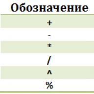
To perform calculations in any cell of the table, you must create inside it the simplest formula, which must always begin with an equal sign (=). To specify mathematical operations inside a formula, ordinary arithmetic operators are used:

For example, let's imagine that we need to add two numbers - "12" and "7". Place the mouse cursor in any cell and type the following expression: "=12+7". At the end of the input, press the "Enter" key and the result of the calculation - "19" will be displayed in the cell.
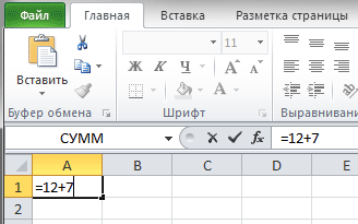

To find out what a cell actually contains - a formula or a number - you need to select it and look at the formula bar - the area immediately above the column names. In our case, it just displays the formula that we just entered.
After carrying out all the operations, pay attention to the result of dividing the numbers 12 by 7, which turned out to be not integer (1.714286) and contains quite a few digits after the decimal point. In most cases, such precision is not required, and such long numbers will only clutter up the table.
To fix this, select the cell with the number for which you want to change the number of decimal places after the decimal point and on the tab home in Group Number select a team Decrease bit depth. Each press of this button removes one character.
To the left of the team Decrease bit depth there is a button that performs the reverse operation - increases the number of decimal places to display more accurate values.
Drawing up formulas
Now let's go back to the budget spending table we created in the first part of this series.
.png)
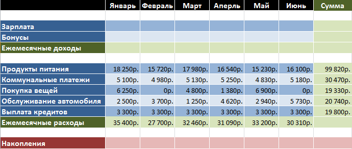
At the moment, it records monthly personal expenses for specific items. For example, you can find out how much was spent in February on food or in March on car maintenance. But the total monthly expenses are not indicated here, although these indicators are the most important for many. Let's correct this situation by adding the line "Monthly expenses" at the bottom of the table and calculate its values.

To calculate the total expense for January in cell B7, you can write the following expression: “=18250+5100+6250+2500+3300” and press Enter, after which you will see the result of the calculation. This is an example of the application of the simplest formula, the compilation of which is no different from calculations on a calculator. Unless the equal sign is placed at the beginning of the expression, and not at the end.
Now imagine that you made a mistake when specifying the values of one or more expense items. In this case, you will have to adjust not only the data in the cells indicating the expenses, but also the formula for calculating the total expenses. Of course, this is very inconvenient, and therefore in Excel, when formulating formulas, not specific numerical values are often used, but cell addresses and ranges.
With that in mind, let's change our formula for calculating total monthly expenses.

In cell B7, enter an equal sign (=) and ... instead of manually entering the value of cell B2, click on it with the left mouse button. After that, a dotted selection frame will appear around the cell, which shows that its value is included in the formula. Now type a "+" sign and click on cell B3. Next, do the same with cells B4, B5 and B6, and then press the Enter key, after which the same amount value will appear as in the first case.
Select cell B7 again and look at the formula bar. It can be seen that instead of numbers - cell values, the formula contains their addresses. This is a very important point, since we just built the formula not from specific numbers, but from cell values that can change over time. For example, if you now change the amount of expenses for the purchase of things in January, then the entire monthly total expense will be recalculated automatically. Try it.
Now let's assume that you need to sum up not five values, as in our example, but one hundred or two hundred. As you understand, it is very inconvenient to use the above method of constructing formulas in this case. In this case, it is better to use the special "AutoSum" button, which allows you to calculate the sum of several cells within the same column or row. In Excel, you can count not only the sums of columns, but also rows, so we use it to calculate, for example, total food expenses for six months.

Place the cursor on an empty cell on the side of the required line (in our case it is H2). Then press the button Sum on the bookmark home in Group Editing. Now, let's go back to the table and see what happened.

In the cell we selected, a formula appeared with an interval of cells whose values need to be summed. At the same time, a dotted selection frame appeared again. Only this time it frames not one cell, but the entire range of cells, the sum of which needs to be calculated.
Now let's look at the formula itself. As before, the equals sign comes first, but this time it is followed by function"SUM" is a predefined formula that will add the values of the specified cells. Immediately after the function there are brackets located around the addresses of the cells whose values need to be summed, called formula argument. Please note that the formula does not contain all the addresses of the summed cells, but only the first and last. A colon between them indicates that range cells from B2 to G2.
After pressing Enter, the result will appear in the selected cell, but this button's capabilities Sum do not end. Click on the arrow next to it and a list will open containing functions for calculating the average values (Average), the number of data entered (Number), maximum (Maximum) and minimum (Minimum) values.

So, in our table, we calculated the total expenses for January and the total food expenses for six months. At the same time, they did this in two different ways - first using cell addresses in the formula, and then using functions and ranges. Now, it's time to finish the calculations for the remaining cells, having calculated the total costs for the remaining months and expense items.
Autocomplete
To calculate the remaining amounts, we will use one remarkable feature of the Excel program, which is the ability to automate the process of filling cells with systematized data.
Sometimes in Excel you have to enter similar data of the same type in a certain sequence, such as days of the week, dates, or row numbers. Remember, in the first part of this cycle, in the header of the table, we entered the name of the month in each column separately? In fact, it was completely unnecessary to enter this entire list manually, since the application can in many cases do this for you.
Let's erase all the names of the months in the header of our table, except for the first one. Now select the cell labeled "January" and move the mouse pointer to its lower right corner so that it takes the form of a cross called fill handle. Hold down the left mouse button and drag it to the right.
.png)
A tooltip will appear on the screen, which will tell you the value that the program is going to insert in the next cell. In our case, this is "February". As you move the marker down, it will change to the names of other months, which will help you figure out where to stop. After the button is released, the list will be filled in automatically.
Of course, Excel does not always correctly "understand" how to fill in subsequent cells, since the sequences can be quite diverse. Let's imagine that we need to fill a string with even numerical values: 2, 4, 6, 8, and so on. If we enter the number "2" and try to move the autofill marker to the right, it turns out that the program offers, both in the next and in other cells, to insert the value "2" again.
 In this case, the application needs to provide a little more data. To do this, in the next cell on the right, enter the number "4". Now select both filled cells and again move the cursor to the lower right corner of the selection area so that it takes the form of a selection marker. By moving the marker down, we see that now the program has understood our sequence and shows the required values in the prompts.
Thus, for complex sequences, before using autocomplete, it is necessary to fill in several cells at once, so that Excel can correctly determine the general algorithm for calculating their values.
Now let's apply this useful feature of the program to our table, no matter what we enter the formulas manually for the remaining cells. First, select the cell with the amount already calculated (B7).

Now "hook" the cursor on the lower right corner of the square and drag the marker to the right to cell G7. After you release the key, the application itself will copy the formula into the marked cells, while automatically changing the addresses of the cells contained in the expression, substituting the correct values.
Moreover, if the marker is moved to the right, as in our case, or down, then the cells will be filled in ascending order, and to the left or up - in descending order.
There is also a way to fill a row with a ribbon. Let's use it to calculate the sums of expenses for all expenditure items (column H).

We select the range to be filled, starting from the cell with the already entered data. Then on the tab home in Group Editing press the button Fill and choose the direction of filling.
Adding Rows, Columns, and Merging Cells
To get more practice in formulating formulas, let's expand our table and at the same time learn a few basic formatting operations. For example, let's add income items to the expenditure side, and then we will calculate possible budget savings.
Suppose that the income part of the table will be located on top of the expenditure part. To do this, we will have to insert a few additional lines. As always, there are two ways to do this: using commands on the ribbon or using the context menu, which is faster and easier.
Click in any cell of the second row with the right mouse button and in the menu that opens, select the command Insert… and then in the window - Add line.
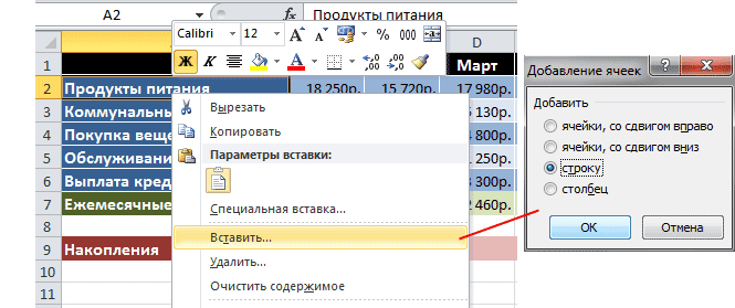
After inserting a row, note the fact that by default it is inserted above the selected row and has the format (cell background color, size settings, text color, etc.) of the row above it.

If you want to change the default formatting, right after pasting, click on the button Add Options, which will automatically appear next to the bottom right corner of the selected cell, and select the option you want.
By a similar method, columns can be inserted into the table, which will be placed to the left of the selected one and individual cells.
By the way, if in the end a row or column ends up in an unnecessary place after insertion, they can be easily deleted. Right-click on any cell belonging to the object to be deleted and in the menu that opens, select the command Delete. Finally, specify what exactly needs to be deleted: a row, a column, or a single cell.
You can use the button on the ribbon for adding operations. Insert located in the group cells on the bookmark home, and for removal, the command of the same name in the same group.
In our case, we need to insert five new rows at the top of the table right after the header. To do this, you can repeat the addition operation several times, or you can use the “F4” key after performing it once, which repeats the most recent operation.
As a result, after inserting five horizontal rows at the top of the table, we bring it to the following form:
We left white unformatted rows in the table on purpose in order to separate the income, expenditure and total parts from each other by writing the appropriate headings in them. But before we do that, we will learn one more operation in Excel - cell merging.
When merging several adjacent cells, one is formed, which can occupy several columns or rows at once. In this case, the name of the merged cell becomes the address of the top maiden cell of the merged range. At any time, you can split a merged cell again, but a cell that has never been merged cannot be split.
When merging cells, only the top left data is saved, while the data of all other merged cells will be deleted. Keep this in mind and it's better to merge first, and only then enter the information.
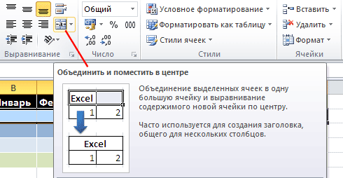
Let's go back to our table. In order to write headings in white lines, we need only one cell, while now they consist of eight. Let's fix this. Select all eight cells of the second row of the table and on the tab home in Group alignment click the button Merge and center.
After executing the command, all selected cells in the row will be merged into one large cell.
There is an arrow next to the merge button, clicking on which will bring up a menu with additional commands that allow you to: merge cells without center alignment, merge entire groups of cells horizontally and vertically, and also unmerge.
After adding headers, as well as filling in the lines: salary, bonuses and monthly income, our table began to look like this:

Conclusion
In conclusion, let's calculate the last line of our table, using the knowledge gained in this article, the calculation of the cell values of which will occur according to the following formula. In the first month, the balance will consist of the usual difference between the income received for the month and the total expenses in it. But in the second month, we will add the balance of the first month to this difference, since we are calculating savings. Calculations for subsequent months will be carried out according to the same scheme - accumulations for the previous period will be added to the current monthly balance.
Now let's translate these calculations into formulas understandable by Excel. For January (cell B14), the formula is very simple and will look like this: "=B5-B12". But for cell C14 (February), the expression can be written in two different ways: “=(B5-B12)+(C5-C12)” or “=B14+C5-C12”. In the first case, we again calculate the balance of the previous month and then add the balance of the current month to it, and in the second, the already calculated result for the previous month is included in the formula. Of course, using the second option to build a formula in our case is much more preferable. After all, if you follow the logic of the first option, then in the expression for the March calculation there will already be 6 cell addresses, in April - 8, in May - 10, and so on, and when using the second option, there will always be three of them.
To fill in the remaining cells from D14 to G14, we use the ability to automatically fill them, just as we did in the case of the amounts.
By the way, to check the value of the final savings for June, located in cell G14, in cell H14 you can display the difference between the total amount of monthly income (H5) and monthly expenses (H12). As you can see, they must be equal.
As can be seen from the latest calculations, formulas can use not only the addresses of adjacent cells, but also any other, regardless of their location in the document or belonging to a particular table. Moreover, you have the right to link cells located on different sheets of the document and even in different books, but we will talk about this in the next publication.
And here is our final table with the calculations performed:

Now, if you wish, you will be able to continue filling it on your own, inserting both additional items of expenses or income (rows) and adding new months (columns).
In the next article, we will talk in more detail about functions, deal with the concept of relative and absolute links, be sure to master a few more useful table editing elements, and much more.
In continuation, I will tell you how to work in Microsoft Excel, a spreadsheet included in the Microsoft Office package.
The same principles of work that we will look at here apply to the free WPS Office package discussed in the previous lesson (if you do not have Microsoft Office on your computer).
There are a lot of sites on the Internet dedicated to working in Microsoft Excel. The possibilities of spreadsheets, which include Excel, are very large. Perhaps that is why, with the release in 1979 of the first such program, which was called VisiCalc, for the Apple II microcomputer, they began to be widely used not only for entertainment, but also for practical work with calculations, formulas, and finances.
In order to start the first steps in order to understand the principle of working in Excel, I offer this lesson.
You may object to me - why do I need Excel for home calculations, a standard calculator is enough, which is in. If you add two or three numbers, I agree with you. What is the advantage of spreadsheets, I'll tell you.
If we, entering several numbers, notice an error on the calculator, especially at the beginning of the input, we need to erase everything that was typed before the error and start typing again. Here we can correct any value without affecting others, we can calculate a set of values with one coefficient, then change only it, with another. I hope I convinced you that this is a very interesting program that is worth getting to know.
Launching Microsoft Excel
To start the program, click the button - Start - All Programs - Microsoft Office - Microsoft Excel (if you have a free WPS Office package - Start - All Programs - WPS Office - WPS Spreadsheets).
In order to enlarge the image, click on the picture with the mouse, return - one more click
The program window fig.1 opens. Just like Word, you can select several areas - they are marked with numbers.
- Tabs.
- Tab tools.
- Sheet navigation area.
- Formula area.
- Columns.
- Strings.
- Page layout area.
- Image scale.
- The workspace of the sheet.
- Book navigation area.
Now a little more.
Excel is called a spreadsheet because it is basically a table with cells at the intersection of columns and rows. Each cell can contain different data. The data format can be:
- text
- numerical
- monetary
- time
- percentage
- booleans
- formulas
The text, as a rule, is necessary not for the calculation, but for the user. In order for the data in the cell to become text, it is enough to put an apostrophe at the beginning of the line - '. What happens after the apostrophe will be treated as a string, or select the “Text” cell format. Fig.2 
Numbers are the main object on which calculations are made. fig.3 
Date and Time - Displays the date and time. Dates can be calculated. fig.4 (different display formats) 
Boolean values can take two values - "True (True)" and "False (False)". When used in formulas, depending on the logical value, you can perform different branches of calculations. fig.5 
Formulas in cells are needed directly for calculations. As a rule, in the cell where the formula is located, we see the result of the calculation, we will see the formula itself in the formula bar when we stand on this cell. The formula starts with the '=' sign. For example, let's say we want to add the number in cell A1 to the number in cell B1 and place the result in cell C1. We write the first number in cell A1, the second in B1, in cell C1 we write the formula ”=A1+B1” (A and B on the English keyboard layout) and press. In cell C1 we see the result. We return the cursor to cell C1 and in the formula bar we see the formula. Fig.6 
By default, the cell format is - general, depending on the entered value, the program tries to determine the value (except when we put an apostrophe (‘) or equals (=) at the beginning).
The numbers 5 and 6 in Fig. 1 indicate the columns and rows of our table. Each cell is uniquely identified by a column letter and a row number. The cursor in Fig. 1 is in the upper left corner in cell A1 (displayed in the navigation area under the number 3), next to the right is B1, and from A1 next down is A2. fig.7 
An example of working in Microsoft Excel
The easiest way to learn how to work in Excel is to learn by example. Let's calculate the monthly rent. I must say right away that the example is conditional, the tariffs and volumes of consumed resources are conditional.
Put the cursor on column A, Fig. 8,  and click on it with the left mouse button. In the menu that opens, click on the item "Format Cells ...". In the next menu that opens, Fig. 9
  On the "Number" tab, select "Text". In this column we will write the name of the service.
From the second line we write:
Electricity
Cold water
Export of solid waste
Heating
Our inscriptions go to column B. We put the cursor on the border between columns A and B, it turns into a dash with two arrows left and right. We press the left mouse button and, moving the border to the right, increase the width of column A fig.10. 
Having placed the cursor on column B, press the left mouse button and, moving to the right, select columns B, C, D. By clicking on the selected area with the right mouse button Fig. 11,  in the menu that opens, on the “Number” tab, select the “Numeric” format.
In cell B1 we write “Tariff”, in C1 “Volume”, D1 “Amount” Fig.12. 
In cell B2, of the “Electricity” tariff, we enter the tariff, in cell C2, the volume, the number of kilowatts of electricity consumed.
In B3, the tariff for water, in C3, the volume, the number of cubic meters of water consumed.
In B4, the tariff for the removal of solid waste, in C4, the area of the apartment (if the tariff depends on the area, or the number of residents, if the tariff depends on the number of people).
In B5, the tariff for heat energy, in B5, the area of the apartment (if the tariff depends on the area).
We become in cell D2 Fig. 13,  write the formula “=B2*C2” and press. The result of Fig.14 appears in cell D2.
  We return to cell D2 Fig.15.
  We move the cursor to the lower right corner of the cell, where the dot is. The cursor turns into a cross. Press the left mouse button and drag the cursor down to cell D5. We copy formulas from cell D2 to cell D5, and we immediately see the result of Fig. 16 in them.
  In cell D2, we wrote the formula “=B2*C2”, if we go to cell D3 in Fig. 17,
  we will see that when copying in the formula bar, it has changed to “=B3*C3”, in cell D4, there will be a formula “=B4*C4”, in D5, “=B5*C5”. These are relative links, about absolute ones, a little later.
We wrote the formula by hand. I will show another way to introduce the formula. Let's calculate the final result. We put the cursor in cell D6 in order to insert the total formula there. In the formula bar of Fig.18,  left-click on the function label, marked with the number 1, in the menu that opens, select the “SUM” function, marked with the number 2, at the bottom (highlighted with the number 3) there is a hint what this function does. Next, click "OK". The function arguments window is opened Fig.19,
  where by default the range of arguments for summation is proposed (numbers 1, 2). If the range suits us, click “OK”. As a result, we get the result of Fig.20.
You can save the book under any name. The next time, to find out the amount, just open it, enter the consumption volumes for the next month, and we will immediately get the result.
Absolute and relative links
What are absolute and relative links. We encountered relative links in the previous example. When we copied the formula, our cell addresses from the formula changed in accordance with the change in rows. A relative reference is written as A1 or B5.
Now we will look at another example.
Let's type a list of fruits, price, weight, amount, discount amount, discount amount, discount.
Let's fill in the table in Fig.21.  For the sum in column D, we will type the sum formula, and copy it as in the previous example. Let's put a discount in cell C2, let's say 15%. Now let's write the formula for the discount amount in cell F2. If we write “=D2*G2”, then when copying in the 3rd line of formulas, it will be “=D3*G3”, and the percentage of the discount is in cell “G2”, and in cell “G3” is empty. In order for the formula to copy the reference to the cell “G2” and there is an absolute addressing.
To do this, a dollar sign is placed in front of the column and row names. It looks like this - "$G$2". Let's try to write the formula “=D2*$G$2” like this and then copy Fig.22.  Let's put the cursor in cell F3 (marked with the number 1) Fig. 23,
  in the formula bar we see the formula “=D3*$G$2” (marked with the number 2), i.e. what we need. Well, now we can write the formula for the discounted amount “=D2-D2*$G$2” (number 2) fig.23.
There is another type of links - mixed. When the dollar sign appears only before a column name or only before a row name.
Little trick. Sometimes it is necessary to number a list in Microsoft Excel. There are several ways to do this. I will show one of them. Suppose we have a list of Fig.24.  Right-click on column A, select “Paste” from the menu that opens. Select the new column in Fig. 27 and set the alignment in the middle and alignment in the center. In cell A1 we put the number 1, in A2 we put the number 2. Select these two cells, become the cursor in the lower left corner of Fig. 25
  (on a dot), the cursor turns into a cross, and drag down to the end of the list. Release the mouse button - the list is numbered Fig. 29
This data is enough to start working in Microsoft Excel. This is the purpose of this lesson.
Excel is one of the most powerful applications in the entire Office suite. It is used not only by accountants and economists, but also by ordinary people. The program is designed to work with numbers and tables, it makes it possible to present information in the most favorable form for perception: as diagrams and graphs. Here you can carry out complex calculations and perform various mathematical operations. In addition, the user does not need special knowledge, it is enough to learn how to work in Excel.
What is this office application?
The Excel program works with files that form a kind of book, consisting of separate sheets. Letters, symbols and numbers are entered into table cells. They can be copied, moved or deleted. If necessary, various operations are carried out with them: text, mathematical, logical and others. Beginners who are just learning how to work in Excel should know that any information can be displayed in the form of graphs or charts.

How to create a file?
First of all, you need to open the document. To create it, you need to click on the program shortcut or go to the application through the "Start".
The default name is Book 1, but you can enter any name in the File Name field. When working, it is worth periodically saving data to avoid losing information in the event of a computer crash or freeze.
You can easily switch between sheets by clicking on the corresponding inscription at the bottom of the page. If there are a lot of tabs, it is better to use the arrow keys on the keyboard. To insert a sheet, you need to find the item "Insert" in the "Home" menu. All possible actions applicable to sheets, such as add or delete, will be displayed there. You can also move tabs around.
"Face" of the program
Before you figure out how to work in Excel, it's worth learning the interface. The tools are located at the top and bottom of the window, and the rest of the area is occupied by rectangles, which are cells. A feature of spreadsheets is that actions can be performed in some cells, and the result can be displayed in others.
Each table has columns, which are denoted by letters of the English alphabet. Lines are numbered on the left. Thus, any cell has its own coordinates. In each cell, you can enter both data and formulas. Before entering the latter, you must put the symbol "=".
Each cell has its own characteristic
To understand how to learn how to work in Excel correctly, the user must know that before entering values, it is necessary to set the dimension of a column or cell. It will depend on how the data is measured. To do this, right-click on the selected range and select "Format Cells" in the dialog box.
If the input number is greater than 999, you must set the split by digits. You don't have to enter spaces yourself.
To correctly display data, you cannot enter more than one single value in one cell. Also, do not enter enums separated by commas or other characters. Each value must have its own cell.

How to enter data?
It will not be difficult for users who know to enter data. To do this, click on the cell and type letters or numbers on the keyboard. To continue working, you must press "Enter" or TAB. A line break is performed using the ALT + "ENTER" combination.
When entering a month or a number in order, it is enough to write the value in the initial cells, and then drag the marker to the required range.
Text wrap
Most often, users are interested in how to learn how to work with text in Excel. If necessary, it can be transferred word by word. To do this, you need to select certain cells and in the "Home" tab you need to find the "Alignment" option, and then select "Text Wrap".
If you want to automatically change the width and height of the cell according to the entered text, do the following: go to the "Home" tab and in the "Cells" group select the "Format" item. Next, you need to choose the appropriate action.
Formatting
To format numbers, you need to select the cell and in the "Home" tab find the "Number" group. After clicking on the arrow next to the "General" item, you can select the desired format.
To change the font, you need to select a specific range and go to the "Home", "Font" menu.
How to create a table?
Knowledge of how to work in the Excel program is unlikely to be useful to the user if he does not know how to create a table. The easiest way is to select a certain range and mark the borders with black lines by clicking on the corresponding icon at the top of the page. But often a non-standard table is required for forms or documents.
First of all, you need to decide how the table should look in order to set the width and length of the cells. With the range selected, go to the Format Cells menu and select Alignment. The "Merge Cells" option will help remove unnecessary borders. Then you need to go to the "Borders" menu and set the required parameters.
Using the Format Cells menu, you can create different variations of tables by adding or removing columns and rows, as well as changing borders.
Knowing how to work in an Excel spreadsheet, the user will be able to create headings. To do this, in the "Table formatting" box, check the box next to the "Table with headers" item.
To add elements to the table, you must use the "Designer" tab. There you can select the required options.

What are macros for?
If a user often has to repeat the same actions in a program, knowledge of how macros work in Excel will be useful to him. They are programmed to perform actions in a specific sequence. The use of macros allows you to automate certain operations and facilitate monotonous work. They can be written in different programming languages, but their essence remains the same.
To create a macro in this application, you must enter the "Tools" menu, select the "Macro" item, and then click "Start Recording". Next, you need to perform those actions that are often repeated, and after finishing work, click "Stop Recording".

All these instructions will help a beginner figure out how to work in Excel: keep records, create reports, and analyze numbers.
This program is used by a large number of people. Andrey Sukhov decided to record a series of educational video lessons "Microsoft Excel for Beginners" for novice users and we invite you to familiarize yourself with the basics of this program.
Lesson 1
In the first lesson, Andrey will talk about the interface of the Excel program and its main elements. You will also understand the workspace of the program, with columns, rows and cells. So here's the first video:
Lesson 2: How to Enter Data in an Excel Spreadsheet
In the second video tutorial on the basics of Microsoft Excel, we will learn how to enter data into a spreadsheet, and also get acquainted with the auto-fill operation. I think that the most effective learning is the one built on practical examples. So we will begin to create a spreadsheet that will help us maintain a family budget. Based on this example, we will consider the tools of the Microsoft Excel program. So here's the second video:
Lesson 3. How to format spreadsheet cells in Excel
In the third video tutorial on the basics of Microsoft Excel, we will learn how to align the contents of the cells of our spreadsheet, as well as change the width of the columns and the height of the rows of the table. Next, we will get acquainted with the Microsoft Excel tools that allow you to merge table cells, as well as change the direction of text in cells if necessary. So here's the third video:
Lesson 4. How to format text in Excel
In the fourth video tutorial on the basics of Microsoft Excel, we will get acquainted with the text formatting operations. For different elements of our table, we will apply different fonts, different font sizes and text styles. We will also change the text color and set a colored background for some cells. At the end of the lesson, we will get an almost ready-made family budget form. So, the fourth video:
Lesson 5
In the fifth video tutorial on the basics of Microsoft Excel, we will finalize the family budget form that we started working on in previous lessons. In this lesson, we will talk about cell borders. We will set different borders for different columns and rows of our table. By the end of the lesson, we will have a family budget form completely ready for data entry. So, the fifth video:
Lesson 6
In the sixth video tutorial on the basics of Microsoft Excel, we will fill in our family budget form with data. Microsoft Excel allows you to simplify the process of data entry to the maximum, and we will get acquainted with these features. Next, I will talk about data formats in cells and how they can be changed. By the end of the lesson, we will receive a family budget form filled in with initial data. So, the sixth video:
Lesson 7
In the seventh video tutorial on the basics of Microsoft Excel, we will talk about the most interesting thing - about formulas and calculations. Microsoft Excel has a very powerful toolkit for performing various calculations. We will learn how to perform basic calculations using spreadsheets, then we will get acquainted with the function wizard, which greatly simplifies the process of creating formulas for performing calculations. So, the seventh video:
Lesson 8
In the eighth video tutorial on the basics of Microsoft Excel, we will completely finish working on the family budget template. We will compose all the necessary formulas and carry out the final formatting of rows and columns. The family budget form will be ready and if you keep your family budget, you will be able to adjust it to fit your expenses and income. So, the eighth video:
Lesson 9
In the final ninth lesson on the basics of Microsoft Excel, we will learn how to create charts and graphs. Microsoft Excel has a very impressive toolkit for visualizing the results of calculations. In the form of graphs, charts and histograms, you can present any data, both simply entered into a spreadsheet, and data obtained as a result of calculations. So, the final ninth video:
Every Windows user has heard more than once about the MS Office software package, in particular about Excel. Its main function is to work with tables. At first glance, the program environment will seem complicated, but after reading this article, you will understand how simple everything is.
Create a table
To begin with, Microsoft tools (Word, Excel, Publisher and Power Point) must be installed on the computer. An Excel file is created in two clicks. Right-click on the desktop, then select "New" → "Microsoft Excel Sheet". After that, open the file.
At first glance, you intuitively understand that you need to enter values in the table, but this is not enough for us, so we will consider each Excel function separately.
How rows and columns are highlighted
Selection is a standard action that is used for further operations.
Hold the left mouse button on one cell, and move the cursor along the column or row, after completion, release the button.
How to change cell borders
There are times when text or a number won't fit in a cell. According to the physics of the program, an infinite amount of information can be stored in one cell, but to visualize the table, you can increase the columns and rows.
This is done in one step. Top and side of the table - markup. You hold LMB on the border of the markup and drag to adjust the dimensions. 
Advice! If you accidentally spoil a column or row, then use the key combination Ctrl + Z. Thus, you will return the dimensions of the column or row to their original state.
Insert a column or row
In practice, you will definitely come across a moment when you have to insert a row or column in a table. This is done with a couple of steps.
Rows are added only at the top and left. To do this, click on the cell, find the "Insert" section on top and select what you are going to insert (column or line). 
To save time, create multiple columns at the same time. You can select several cells horizontally, then as many rows as you have selected will be added. When selecting vertically, columns are created according to the same principle. 
Advice! The same action can be carried out using key combinations. To do this, select the column, press Ctrl + Shift + "=" and we have an empty column on the left. Similarly, an empty line is created.
Cell merging
We make one from two cells. This action is very quick and easy. Cells can be combined not only horizontally and vertically, but also simultaneously, capturing, for example, two columns vertically and 2 rows horizontally. To do this, select all the necessary cells (at least two) and at the top click on the "Merge and place in the center" button. 
Create a table with formulas
Essentially, Microsoft Excel is built on the application of mathematical formulas. Knowing them, you can easily do any calculations in the table. In order to understand how they are used, elementary examples will be provided to you.
We need to buy 5 folders. One folder costs 20 rubles. Find out the amount that the folders will cost us.

Instead of the multiplication sign (as shown in the example), any sign could be used. You can select more than two coefficients (when working with the "+" and "-" actions). You can also combine actions.
Attention! Any calculations using formulas can only be carried out in one row or in one column!
Creating a dynamic (smart) table
It may sound strange, but in a regular table you can create a "Smart" table. Its essence lies in greater functionality. In it, you can set more interesting formulas, with the help of which the table will become automated.
It is created by simply clicking on the "Format as Table" button. Next, choose a design (you can choose any, in the future it will be possible to change it). Many people think that this function only colors the table, but it is not. After that, your table becomes smart.
Advice! If you are using tables with big data, and a row, column, or some area needs to be visible, use the .
Working with a dynamic table
The range of functions of dynamic tables is huge, so we will focus on the most basic ones.